Machine Learning Based on Neural Network Fitting for Traffic Behaviour at Road Intersection in Mixed Traffic Condition

Acknowledgement

This work was supported by the Ministry of Higher Education, Malaysia FRGS/1/2019/TK08/MMU/03/1 and TMRND Grant MMUE/190012.

Introduction

Annually, average of 1.3 million lives due catastrophic loss on roadways worldwide, meanwhile around 10 million are experience causalities [1]. Recently, the increasing number of researchers concentrating the development of system that can detect or identify the hazardous driving behaviors instantly. In autonomous, the process to recognize the hazardous situation by collection of training data that associate with serious traffic conflicts [2]. This approach, can train the artificial intelligent to improve the risk prevention of autonomous vehicles [3]. Automated vehicle typically assembled with verified controllers’ function to analysis the hazard and strategy to mitigate the hazard [3]. The essential of having these controllers are ability to detect and prevent of hazards in every possible angle or dimension situation. The challenges in autonomous vehicles (AV) are regarding cybersecurity issues and how to protect the AV from cyber-attacks [4]. Despite of having unique password the application of security protocols and supply chain might be the best solution to defend the AV from any disruption.

The near-infrared (NIR) camera sensors technique used to record the driver reaction classification [5]. However, the data collected is less than 30 cases and have limitation for recognizing the driving characteristic. Driver’s Risk Field (DRF) were introduced by (Kolekar et al., 2020), to measure the probability of traffic conflict event by using two-dimensional field [6]. Yet, this method has not practically been practices to detect the reckless driving behavior in real time series. Recently, the study using machine learning algorithms to investigated the reckless driving behavior [7]. The method has ability to detect the hazardous driving behavior automatically by applying the algorithms. This approach has advantage to improve the accuracy of previous algorithms by removing the bias in dataset and refining the quality of data. Intelligent driver model (IDM) study the effect of lighting environment influences the traffic behavior [8]. The outcomes reveal, infrastructure like tunnel lighting and sunscreens at tunnel gateway can improve the traffic flows and avoiding traffic swaying. Recently multi-attention-based Hybrid-Complication Spatial- Time Based Recurrent Network (HRSRN) purpose to predict traffic flow at urban and rural area [9]. The advantage of this system it has ability to capture traffic flow spatial- time based topographies. This method performed good result from previous models in terms of mean absolute error (MAE) and root mean square error (RMSE).

Another visual technique to compute traffic flow, macroscopic analysis, concentration traffic geographies and traffic flow response, call novel traffic flow prediction model, V-STF [10]. The model justifies the improvement of accuracy during non-interrupted peak hours in congested road environments. This method also performed a good result in predicting immediate traffic disruption.

The psychological behavioral data model using deep learning approach propose for driver identification and verification [11]. The approach implementing fully convolution network and excitation block, performed accuracy and verification accuracy of 99.60% and 90.91 respectively. On the top of that, the model effectively distinguishes drivers and frauds detections for the security reasons.

By adopting driving simulator to analyse the different between new and experience drivers [12]. The study reveal, new drivers can only respond operation either braking or steering in the conflict situation. Meanwhile experienced drivers, has abilities to combine both operations at the same time, and to overcome the traffic destruction. Furthermore, experienced drivers can handle difficult situation such as quick respond scanning the safe surrounding to avoid hazardous environment, meanwhile novice driver react opposite. This finding may provide essential perspective for future driving assistance system.

In neuroscience the definition of artificial neural networks (ANNs) are accomplishing human-stage characteristic performance in multiple tasks, including face recognition, language analysing, complex gameplay, and motor learning [13-16]. Previous study found the automotive industry, construction and road safety are dominant applying of machine learning algorithms for risk valuation. Meanwhile in engineering risk assessment, artificial neural networks are the leading method for machine learning [17]. Figure 1, shows the application field of the machine learning in multidisciplinary field including autonomous, traffic prediction, image recognition, medical diagnosis, speech recognition, fraud detection, automatic language translation, virtual personal assistant, email spam, stock market trading and product recommendation.

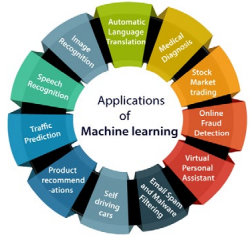
Figure 1: Various Flied Application of Machine Learning

The digital challenge in artificial intelligent directly influence the artificial neural network. Typically, computer function can overcome complex mathematical easily compare to human capability. However, it has disadvantage in term of solving difficulty problem instantly [18]. The neural architecture basic concept is like human brain and well organize for replying complex questions and so on. The algorithm approach used to duplicating this architecture and be able to answer. In this research, it considers a feed forward single hidden layer neural network [18].

The fundamental of architecture comprise three layers of neurons: the input layer, hidden layer, and output layer. The Input layers normally associate with input variables (i.e., each variable for one neuron). In input layer content weighted flow, w, linked to each variable to each of hidden layer neurons [17]. Furthermore, in hidden layer each neuron is connected by weighted flow, β, and linked to single output layer neuron [18]. The variable X = {x1 + x2 + x3 +......n, function as input variables n, meanwhile m hidden neurons, dichotomous outcomes Y, and function g, the neural network equation can be derived as follows:

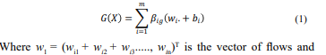
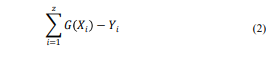
linking the n input neurons to the ith in hidden neuron, βi is the flow connecting the i th hidden neuron to the single output neurons, bi the bias connected with the i th hidden neuron [18]. Provide a dataset with Z total observation, each with predictor set Xi and dichotomous outcomes Yi , the value of wi , βi and bi are found by minimizing the distance between predicted and actual outcomes

The structure of this study was organizing as follow, Section 2 briefly describe the methodology of the study and machine learning. Section 3 focus on neural network fitting and the different between three methods Levenberg-Marquardt Algorithm, Bayesian-Regularization Algorithm and Scaled Conjugate Gradient Algorithm. Next, Section 4 discussion and finally Section 5 finding and conclusion.

Methodology

Federal Route 50, located in the Southern Peninsula of Malaysia, was selected for this study. The design of this infrastructure has four lane and two carriageways with a design speed of 100 km/h. In 2024, it will have the capacity to receive more than 92,000 veh/ day or 9,100 veh/h. Data collection using a video camera at eleven blackspot areas was accomplished, and microscopic analysis of the traffic behavior was performed in the laboratory.

Table 1, summarize the input layer and output layer for ANN model. Input layer represent of 58 attributes. Meanwhile, Output layer consist of right turn motor vehicles (RMV). In the input layer dataset, this study has eight main cluster involved vehicle category (VC), second vehicle passing RMV (SVP), first vehicle passing RMV (FVP), speed limit (SP), gap pattern (GP), infrastructure (Infra), type of conflict (TC) and day time (DT). Speed limit has 20 items: speed limit less than (SP 25kph, SP30kph, SP35kph…n), vehicle category has 7 items: passenger cars, riders, pillions, lorries, and vans. Traffic of conflict has 5 items: angular conflict, rear end conflict, head-on conflict, change lane conflict, motorcycle stop conflict (AGc, REc, Hoc, CLc, and MSc) [19-21]. Infrastructure has 5 items: channelization, traffic signal, median, lane width and pedestrian bridge (Chlzation, TS, Md, Lw, and Pb) [22]. Gap patterns consist 5 items: gap pattern 1, gap pattern 2, gap pattern 3, gap pattern 4 and gap pattern 5 (Gp1, Gp2, Gp3, Gp4 and Gp5) [23]. Second vehicle is passenger car, motorcycle, bus, lorry and van passing the RMV on the major road has 5 items (SCar, SMc, SBus, SLorry, and SVan) [21]. First vehicle is passenger car, motorcycle, bus, lorry and van passing the RMV on the major road has 5 items (FCar, FMc, FBus, FLorry and FVan). Day times has 3 items: morning, midday and afternoon. Meanwhile gap, waiting time and traffic volume, each has 1 item respectively [21].

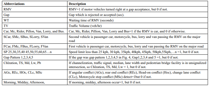
Table 1: Attributes of traffic behaviour models

Machine Learning

In this study MATHLAB R2022b program has been applied and using neural network fitting as a machine learning (ML). They are three category machine learning adopting in this research such as Levenberg-Marquardt Algorithm (LMA), BayesianRegularization Algorithm (BRA) and Scaled Conjugate Gradient Algorithm (SCGA). Subsequently, contrast analysis between those three-machine learning were carried out to justify the outcomes result. First, ANN function to analyse the information from input data, training of network, hidden layer, and output layer. Level of accuracy in the ANN network achieve through continuous training, connection between the units (input layer, hidden layer, output layer) and after the error in the prediction is reduced. The input or predictor data matrix (841 x 58) representing 841 samples of 58 dependent variables. Meanwhile the responses or output data matrix (841 x 1) representing 841 samples of 1 independent variables. The schematic of the neural network was created using neural network fitting. Figure -2 shows a two layer feedforward network consist ten sigmoid hidden neurons and single output layer neural network with one sigmoid suitable for regression task.The simulation involved seventy percent of data (589 samples) was applied for training, fifteen percent (126 samples) used for validating and remining portion was used for testing of the neural network.

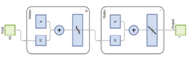
Figure 2: Architecture of the deep neural networks

Results

Neural Network

Fitting As mention before Neural Network Fitting has three methods in Neural Network Fitting function as a Machine Learning. In Levenberg Marquardt Algorithm, mean square error (MSE) has been used to measure the performance of input and output data in the model simultaneously testing the ANN. It means that the significance prediction can be achieved when MSE rate is close to zero, indicate the training performance is good fit or less error.

Figure -3 shows the plot graph between the output rates and input rates. The best validation performance is 0.062527, at alteration 6th. The training process continue until reach alterations 12 and then finish. The graph line for validation and test illustrates the stable flow after reach the alteration 6th except training line diverge after the reach epoch 3.

Next Figure-4 represents the best validating performance is 0.01875, at epochs one thousand by implementing the Bayesian Regularization Algorithm (BRA). The training process stop until meet 1000 alterations. Despite of achieved the lowest error 0.01875, the simulation line between training and test has quite big gap. Both lines recorded steady performance before touch alterations 200. Moreover, this method excluded the validation process.

In Scaled Conjugate Gradient Algorithm (SCGA) as depicted in Figure-5, the best validating performance is 0.0427 which close to zero, at alterations 44. The training run until fifty alterations. Despite of having second best validation performance from other models. Scaled Conjugate Gradient Algorithm represent uniform result of MSE simulation (close to zero) for all three steps training, validating, and testing at epochs 44. This machine learning has been identifying as excellence result for overall steps in the validation performance.

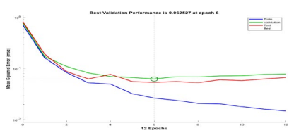
Figure 3: Network Performance for Traffic Characteristic Created with Simulation Data Using Levenberg-Marquardt Algorithm

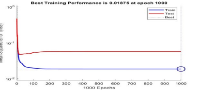
Figure 4: Network Performance for Traffic Characteristic Created with Simulation Data Using Bayesian-Regularization Algorithm

Figure 5: Network Performance for Traffic Characteristic Created with Simulation Data Using Scaled Conjugate Gradient Algorithm

Regression Plot

Figure-6, illustrates the connection between output target values. Typically if the training process is adequate fit, it reflect to output values and target values will achieve same result. Generally, R =1 indicate the prefect regression index between the outputs and the targets. The regression coefficient obtained for tranning, validating, test and all was 0.945, 0.86655, 0.88293 and 0.92391 respectively. The result describes in Levenberg-Marquardt Algorithm (LMA) there is a precision of data fit. Furthermore, it can be explain that the outcomes are acceptable with reasonable errors and the result is close to target. Moreover, the regression between outputs and targets is nearly precise.

Figure 7 shows regression coefficient result for training, test and all was 0.96104, 0.8811 and 0.94848 respectively. The outcomes explain that with Bayesian-Regularization Algorithm, there is a good regression (R close to one) between output and target. Base on three processes in the BRA result perform better regression value than LMA. However, this method does not include validation plot in the process.

Meanwhile Figure 8, by adopting Scaled Conjugate Gradient Algorithm (SCGA) determination of regression coefficient for training, validating, test and all was 0.92047, 0.90798, 0.90403 and 0.91591 respectively. The result indicated an improvement of regression coefficient from previous machine learning and the result nearly to target. All four process in SCGA perform R value above 0.90, which is higher than previous result. Therefore, in average this method can consider as the best performance for four steps of training, validating, testing and all.

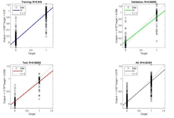
Figure 6: Regression Plot for Traffic Behaviour Model Adopting Levenberg-Marquardt Algorithm

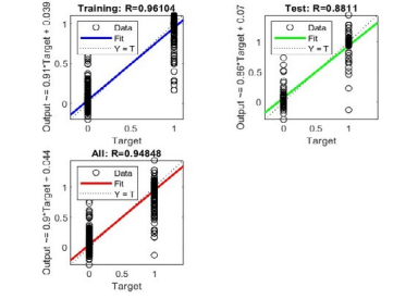
Figure 7: Regression Plot for Traffic Behaviour Model Adopting Bayesian-Regularization Algorithm

Algorithm

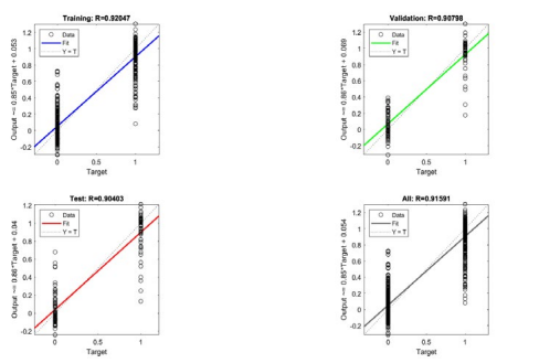
Figure 8: Regression Plot for Traffic Behaviour Model Adopting Scaled Conjugate Gradient Algorithm

MSE and Regression

Table 2 shows the outcomes for training, validation and testing of neural network fitting by adopting Levenberg-Marquardt Algorithm. Mean Squared Error (MSE) defines as average squared variance between outputs and targets. The less values of MSE mean the better result and zero indicate without error. (R) values mean regression, measure the correlation between outputs and targets. An R value typically yield between 0 to 1. Regression (R) value close to 0 mean less relationship, meanwhile ( R = 1) represent prefect relationship. The observation sample of training, validating and test obtained 589, 126 and 126 respectively. Next MSE of training, validating and test stated 0.0242, 0.0847 and 0.0780 respectively. Moreover, R value of training, validating and test record 0.9494, 0.8226 and 0.8412.

Next approach Bayesian Regularization Algorithm, in Table 3 present the result for traning and testing only without validating process. The data observation in this steps involved seven hundred and fifteen for training and one hundred and twenty six for test. Subsequently, the R value for training and test recorded 0.9610 and 0.8811 respectively. Which indicate good correlation between outputs and targets. Furthemore, the MSE result for training and test process was 0.0187 and 0.0577 respectively. It remark the outcomes achived in MSE close to zero value which mean perform good result.

The third mechine learning Scaled Conjugate Gradient Algorithm in Table 4, summarize the outputs for three process training, validating and test. The dataset used in the observation for those three steps was same as Levenberg-Marquardt Algorithm. The R value determine for training, validating and test was 0.9205, 0.9080 and 0.9040 respectively. Meanwhile The MSE value for training, validating and test archived 0.0378, 0.0427 and 0.0451 respectively. The result perform in this method was better than others two approach which recorded R index for all three process above 0.90 and received MSE for all those steps less than 0.05.

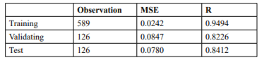
Table 2: Regression (R)Values and Mean Squared Error (MSE) of Neural Network Fitting (Levenberg-Marquardt Algorithm)

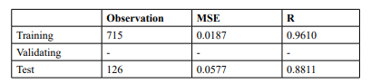
Table 3: Regression (R)Values and Mean Squared Error (MSE) of Neural Network Fitting (Bayesian-Regularization Algorithm)

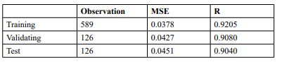
Table 4: Regression (R)Values and Mean Squared Error (MSE) of Neural Network Fitting (Scaled Conjugate Gradient Algorithm)

Error Histogram

Base on the value of MSE (Figure -3) and R (Figure-6) are very close to zero and one, respectively. It explain that the data fitting quite accurate. The error histogram in Figure 9, shows the trained neural network for the tree process of tranning, validating and test. This histogram illustrates that the data fitting errors are well distributed in the accepted range between -0.8569 and 0.9266.

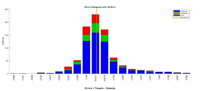
Figure 9:  Error Histogram Of Neural Network Simulation Levenberg-Marquardt Algorithm

In Figure 10, depicted the error histogram using Bayesianregularization algorithm. This machine learning analysis only two process training and test without validation. It indicates that the data fitting errors are also reasonably distributed and fall between -0.6 to 0.9353. This error is reasonably acceptable and qualify for training distribution outcomes.

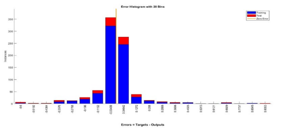
Figure 10: Error Histogram of Neural Network Simulation Bayesian-Regularization Algorithm

The third machine learning Scaled Conjugate Gradient Algorithm as depicted in Figure 10, plot the error histogram. This approach involved three steps training, validating and test. It indicates that the data fitting errors are acceptable sensibly distributed and most error range between -0.9786 to 0.8698. The outcomes from this method are nearly like Levenberg-Marquardt Algorithm.

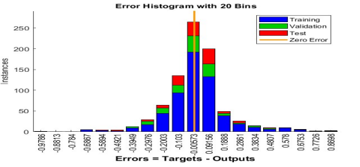
Figure 11: Error Histogram Of Neural Network Simulation Scaled Conjugate Gradient Algorithm

Discussion

In the input predectors data, eight main group has been identify in the traffic behavior dataset. They are vehicle category, second vehicle passing RMV, first vehicle passing RMV, speed limit, gap pattern, infrastructure, type of conflict and day time. The assessment between three machine learning by presenting network visualization simulation, regression algorithm, and error histogram diagram for training, validation and test process may contribute to the present literature, as a domain to traffic safety measure and basic review for autonomous vehicles.

To understand more precise the impact of each variable in the traffic behavior models. It is necessary to develop the models based on eight group in input dataset. The focus group will implement the machine learning and other analytic approach to crystalize the result. In addition, near-infrared (NIR) camera sensors technique, Driver’s Risk Field (DRF), Intelligent driver model (IDM) and Multi-Attention-Based Hybrid-Complication Spatial- Time Based Recurrent Network (HRSRN) are few potential techniques to be explore.

Conclusion

The analysis of Levenberg-Marquardt Algorithm (LMA), Bayesian-Regularization Algorithm (BRA), Scaled Conjugate Gredient Algorithm (SCGA) involved network performance simulation, regression plot and error histogram of neural network simulation. This paper has carried out evaluation between those three mechine learning and revealed that Scaled Conjugate Gradient Algorithm (SCGA) exihibit the best prediction performance for traffic behavior dataset. In average the result for (SCGA) mean square error were below 0.05 and regression value achived more than 0.90 in training, validating and test steps. The finding from this study has significance impact as the proposed approach can be utilized to mechine learning as well as other research flied to determine the highest prediction accuracy.

References

1. Kuupiel, D., Jessani, N. S., Boffa, J., Naude, C., De Buck, E., Vandekerckhove, P., & McCaul, M. (2023). Prehospital clinical practice guidelines for unintentional injuries: a scoping review and prioritisation process. BMC emergency medicine, 23(1), 27.
2. Paterson, C., & Picardi, C. (2023). Hazards help autonomous cars to drive safely.
3. Gleirscher, M. (2017). Run-time risk mitigation in automated vehicles: A model for studying preparatory steps. arXiv preprint arXiv:1709.02560.
4. Alsaade, F. W., & Al-Adhaileh, M. H. (2023). Cyber attack detection for self-driving vehicle networks using deep autoencoder algorithms. Sensors, 23(8), 4086.
5. Naqvi, R. A., Arsalan, M., Rehman, A., Rehman, A. U., Loh, W. K., & Paul, A. (2020). Deep learning-based drivers emotion classification system in time series data for remote applications. Remote Sensing, 12(3), 587.
6. Kolekar, S., Petermeijer, B., Boer, E., de Winter, J., & Abbink, D. (2021). A risk field-based metric correlates with driver’s perceived risk in manual and automated driving: A test-track study. Transportation research part C: emerging technologies, 133, 103428.
7. Yu, L., Zhao, X., Huang, J., Hu, H., & Liu, B. (2023). Research on Machine Learning With Algorithms and Development. Journal of Theory and Practice of Engineering Science, 3(12), 7-14.
8. Yu, S., Zhao, C., Song, L., Li, Y., & Du, Y. (2023). Understanding traffic bottlenecks of long freeway tunnels based on a novel location-dependent lighting-related carfollowing model. Tunnelling and Underground Space Technology, 136, 105098.
9. Zhang, Q., Chang, W., Yin, C., Xiao, P., Li, K., & Tan, M. (2023). Attention-Based Spatial–Temporal Convolution Gated Recurrent Unit for Traffic Flow Forecasting. Entropy, 25(6), 938.
10. Chen, J., Xu, M., Xu, W., Li, D., Peng, W., & Xu, H. (2023). A flow feedback traffic prediction based on visual quantified features. IEEE Transactions on Intelligent Transportation Systems, 24(9), 10067-10075.
11. Xu, J., Pan, S., Sun, P. Z., Park, S. H., & Guo, K. (2022). Human-factors-in-driving-loop: Driver identification and verification via a deep learning approach using psychological behavioral data. IEEE Transactions on Intelligent Transportation Systems, 24(3), 3383-3394.
12. Xu, J., Guo, K., & Sun, P. Z. (2022). Driving performance under violations of traffic rules: Novice vs. experienced drivers. IEEE Transactions on Intelligent Vehicles, 7(4), 908- 917.
13. Taigman, Y., Yang, M., Ranzato, M. A., & Wolf, L. (2014). Deepface: Closing the gap to human-level performance in face verification. In Proceedings of the IEEE conference on computer vision and pattern recognition (pp. 1701-1708).
14. Radford, A., Wu, J., Child, R., Luan, D., Amodei, D., & Sutskever, I. (2019). Language models are unsupervised multitask learners. OpenAI blog, 1(8), 9.
15. Jaderberg, M., Czarnecki, W. M., Dunning, I., Marris, L., Lever, G., Castaneda, A. G., ... & Graepel, T. (2019). Humanlevel performance in 3D multiplayer games with populationbased reinforcement learning. Science, 364(6443), 859-865.
16. Levine, S., Pastor, P., Krizhevsky, A., Ibarz, J., & Quillen, D. (2018). Learning hand-eye coordination for robotic grasping with deep learning and large-scale data collection. The International journal of robotics research, 37(4-5), 421-436.
17. Jain, A. K., Mao, J., & Mohiuddin, K. M. (1996). Artificial neural networks: A tutorial. Computer, 29(3), 31-44.
18. Lolli, F., Gamberini, R., Regattieri, A., Balugani, E., Gatos, T., & Gucci, S. (2017). Single-hidden layer neural networks for forecasting intermittent demand. International Journal of Production Economics, 183, 116-128.
19. Mustakim, F., Ahmad, M. N., Kadir, R. A., Sulaiman, R., Ahmad, A., Aziz, A. A. D., & Mahmud, A. (2023). Ontologies for Supporting Traffic Behaviour, Critical Gap, and Conflict Models at Unsignalized Intersection Routes. Journal of Humanities & Social Sciences, 6(7), 195-213.
20. Mustakim, F., Aziz, A. A., Ahmad, M. N., & Jamian, S. B. (2023). Sustainable Hydrodynamic of Artificial Neural Networks and Logistic Regression Model to Lane Change Serious Conflict at Unsignalized Intersection on Malaysia’s Federal Route. J Curr Trends Comp Sci Res, 2(3), 243.
21. Mustakim, F., Aziz, A. A., Siong, L. H., Bakhuraisa, Y., Rahman, N. Z. B. A. (2024). Impact of Traffic Characteristic at Unsignalized Intersection in Mixed Traffic Condition using Logistic Regression Method (LRM) and Artificial Neural Network (ANN). J Sen Net Data Comm, 4(2), 01-15.
22. Mustakim, F., Aziz, A. A., Mahmud, A., Jamian, S., Hamzah, N. A. A., & Aziz, N. H. B. A. (2023). Structural Equation Modeling of Right-Turn Motorists at Unsignalized Intersections: Road Safety Perspectives. International Journal of Technology, 14(6).
23. Fajaruddin, M., Fujita, M., & Wisetjindawat, W. (2013). Analysis of Fatal-Serious Accidents and Dangerous Vehicle Movements at Access Points on Malaysian Rural Federal Roads. Journal of Japan Society of Civil Engineers, Ser. D3 (Infrastructure Planning and Management), 69(4), 286-299.