Control System for a Local Network of Renewable Energies: Solar-Wind-H2. Simulation and Evaluation of the Operational Process

Introduction

In past decades, the planet has experimented with a global transformation process characterized by population and economic growth without precedents. This process has represented a drastic increase in the World's energy demand, representing a challenge to society's sustainability and environmental protection [1-4]. In human history, fossil fuels have played a significant role in supplying energy for people's activities in the industry, agriculture, and transportation sectors, protecting against adverse meteorological situations since ancient times [5-9].

Fossil fuels, also called “brown power sources”, have been the principal source of energy supply in the last two centuries, revealing as a reliable source to cover industrial, commercial, and residential human needs [10-11]. Despite their high specific weight in human development during the XIX and XX centuries, their undoubted contribution to GHG emissions and global warming makes them a risky business for the planet and environment sustainability [12-14]. Furthermore, fossil fuels are finite and cannot be easily replaced at the rhythm of humankind using them therefore, an energy transition to sustainable sources and more respect for the environment is a must [15-22].

Renewable energies appear as the alternative to fossil fuels; nevertheless, they suffer from low power density, variability, and intermittency, which generates rejection of their adoption as primary sources [23-26]. Hybridization emerges as a solution for solving the renewable energy source intermittency and variability, a common technique that offers advantages and drawbacks like lack of reliability, increasing investment costs, system management, and energy generation surplus [27-32].

In this work, we propose hybridizing solar photovoltaic, wind energy, and hydrogen resources, designing a control system for efficiently managing the power supply and grid integration. The paper’s goal is the optimization of the renewable energy resource use, considering key parameters like the fluctuating energy demand, the energy conversion efficiency, and transmission and distribution power losses [33-34].
 

The approach proposed in this study deals with mitigating environmental problems arising from carbon emissions from using conventional energy sources, such as fossil fuels, aiming to significantly increase the overall efficiency of the global energy system and promote its long-term sustainability. This strategy looks to establish a new paradigm in the management and use of renewable energies, oriented towards an optimization that considers both current energies needs and the preservation of the environment and the well-being of future generations.

Despite this work focuses on consolidated renewable energies like solar, wind, and hydrogen, because of their relevance in the global energy scenario, the frame and methodology proposed in this study extends to a high range of hybrid energy source configurations, both renewable and conventional. The work's structure is adaptive to a variable number of energy sources, showing an extreme flexible capacity of adjustment to any kind of energy systems, and to a more.

diversified energy mix model. The proposed technique allows a quick response to changes in the energy matrix, and promotes a more efficient use of the available energy resources, managing the future energy challenges in a flexible and integrating way.

Fundamentals

Solar thermal power plant

The solar system is a tower-type thermal power plant, which receives concentrated solar radiation into the tower spot from the heliostats distributed in the solar field. Incoming solar radiation is determined using the classical expression [35]:

k_t is the turbidity index, I_so is the solar constant, E_o is the eccentricity of the earth's orbit, δ is the declination, φ is the location latitude, and α is the solar altitude.

The solar constant is a setup parameter, while the earth's orbit eccentricity and declination depend on the year's day. The turbidity index depends on the climatic conditions of the location and can be estimated using predicting models [36-38]. The location latitude depends on the geographical position on the earth's surface, and the solar altitude is a variable parameter depending on latitude and declination as in:

The solar radiation strikes the heliostat mirror and reflects to the tower spot. Since many heliostats contribute to the concentrated solar radiation arriving at the tower spot, the collected power, P_S, is:

ρ_h and S_h are the heliostat mirror reflectivity and surface, N is the heliostat number in the solar field, and F_sp is the spillage factor, which considers the fraction of reflected solar rays that do not intercept the tower spot.

Because a solar thermal power plant operates with a thermodynamic cycle, currently a Rankine cycle, the solar power converts into thermal energy according to the cycle efficiency; therefore, the available power is:

η_th is the thermodynamic cycle efficiency.

Combining all above equations:

The latitude is fixed if we select a specific location on the earth's surface. Other setup parameters are the thermodynamic cycle efficiency, which may be considered constant within a narrow margin around the reference value if operating conditions do not change much, the heliostat reflectivity, surface and elements number, the solar constant, the earth's eccentricity because the deviation regarding the yearly average value is minimum [39-41]. The turbidity index is also constant since the climatic conditions are specific for the area where the power plant is built. Although the spillage factor depends on daytime, it is a common practice to consider this parameter as constant if the solar thermal power plant operating conditions remain unchanged [43-44]. Therefore, the only remaining variable parameter in equation 5 is the declination, which may be expressed as a function of the year's day:

where d is the Julian day. Now, replacing in equation 5, and grouping constant parameters:

Wind Farm

The wind farm power generation derives from the wind energy, which depends on wind speed as in [45]:

ρair is the air density, S_wt is the wind turbine area, and u is the wind speed.

Since the energy suffers a mechanic-electric conversion at the wind turbine, the output power is:

C_p is the wind turbine power coefficient, and η_t and η_g are the mechanic transmission system and electric generator efficiency.

Despite the mechanic transmission system and electric generator efficiency change with operating conditions, the variation is low, and we may consider both parameters as constant within reasonable accuracy [46-47].

The wind resource is erratic and random; therefore, we cannot predict its behavior as in solar radiation. Nevertheless, wind resource can be estimated using modeling from the Weibull distribution, which predicts the wind speed according to a probability function of the type:

λ and κ are the Weibull distribution parameters, and x represents the wind speed interval in the Weibull distribution curve [49].

Since the λ and κ parameters depend on the location, once we build the wind park, λ and κ are fixed; therefore, the wind speed occurrence probability for a specific value, on which the wind power depends.

Energy Generation Form Hydrogen

Hydrogen is an energy vector that requires a transformation process using a conversion system to obtain electric energy. Hydrogen comes from hydrocarbon reforming, gas or petrol processing, methanol or water electrolysis [50-57]. This last process is the most respectful to the environment since the chemical reaction residue is water vapor and is compatible with renewable energy sources [58,59]. The electrolysis/hydrolysis process responds to a double oxidation/ reduction chemical reaction of the type [60-61]:

The electrolysis occurs in an electrolyzer where the electric current decomposes the water molecule in hydrogen and oxygen, as in equation 11. Hydrolysis develops in a fuel cell, combining molecular hydrogen and oxygen to produce water vapor (equation 12). The generated electrons at the electrolysis process represent the electric current used as a power supply for external applications. The electrolysis and hydrolysis process develop at moderately high efficiency, between 60% and 80%, resulting in a combined efficiency in the 40% to 60% range [62]; therefore, we should express the fuel cell output power as:

ηcell is the fuel cell efficiency, n_H2 is the hydrogen molecular flow, and â??H is the hydrogen combustion enthalpy, with a value for the hydrogen â??H = 285 kJ/mole.

Since the electrolysis/hydrolysis process develops at low voltage and current, it is critical to group fuel cell in series and parallel to achieve the required output power; the number of cells in the series or parallel string depends on the output voltage and current. The fuel cell stack layout is, therefore (Figure 1):

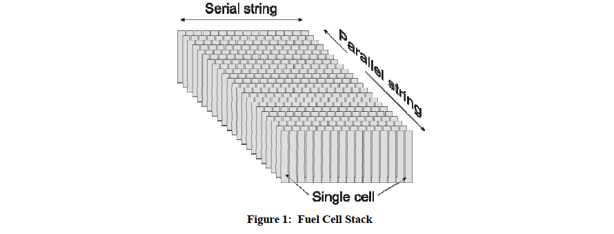
The fuel cell stack global output power is:

Project Project

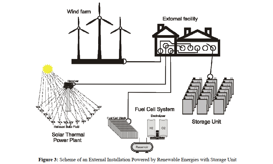
The combined power generation from the three energy sources, solar thermal, wind, and hydrogen, depends on the availability of the renewable resource to produce the required power; indeed, solar thermal depends on solar radiation, which is variable and intermittent, wind resource is erratic and random, and hydrogen requires a renewable source if the electrolysis develops preserving the environment. If the global power generation is not enough to cover energy demand, two solutions arise: importing power from the grid or a storage system; the first solution is technically less complex but depends on grid connection, which is not always available; the second requires a more complicated design and additional elements like the storage unit and DC/DC and DC/AC converters to adapt output current from the renewable sources. Figure 2 shows the schematic representation of an external installation powered by a renewable energy mix with a grid connection.

Figure 3 shows the same installation scheme replacing the grid connection by a storage unit.
 

System Configuration

a) Solar Thermal Power Plant

Solar Thermal Power Plant configuration responds to a classical design with a heliostat solar field that reflects the solar radiation to the receiver. A water heat exchanger converts the concentrated solar radiation into thermal energy, transforming liquid water into vapor that powers a turbine connected to an electric generator to produce electricity, which is carried to the external facility.
 

If the solar plant requires operating beyond sunset, we need a thermal storage unit to accumulate the daily energy surplus so the system continues working for some time after dark. The storage unit is of the molten salt type and provides extra working time depending on size and accumulated energy.

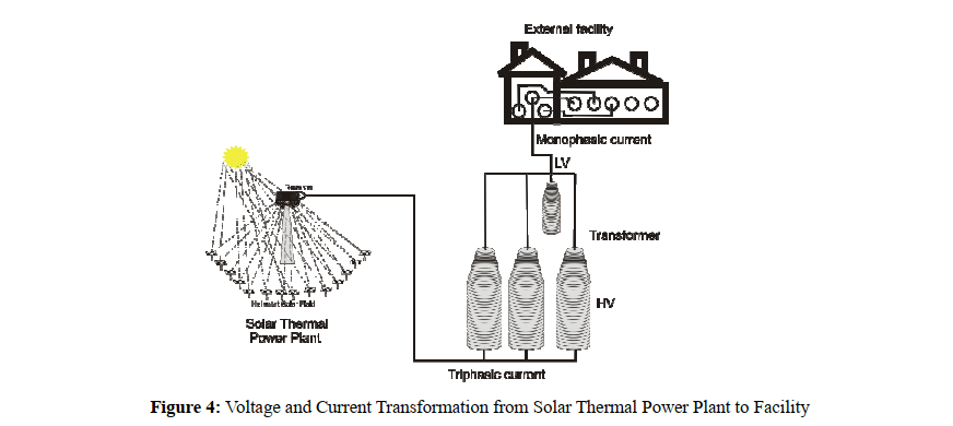
Since solar thermal power plant output does not match the external facility current type and voltage value, we insert an AC transformer to reduce voltage and convert triphasic to monophasic current to make it compatible with external installation appliances. Figure 4 shows the schematic representation.
 

b) Wind Farm

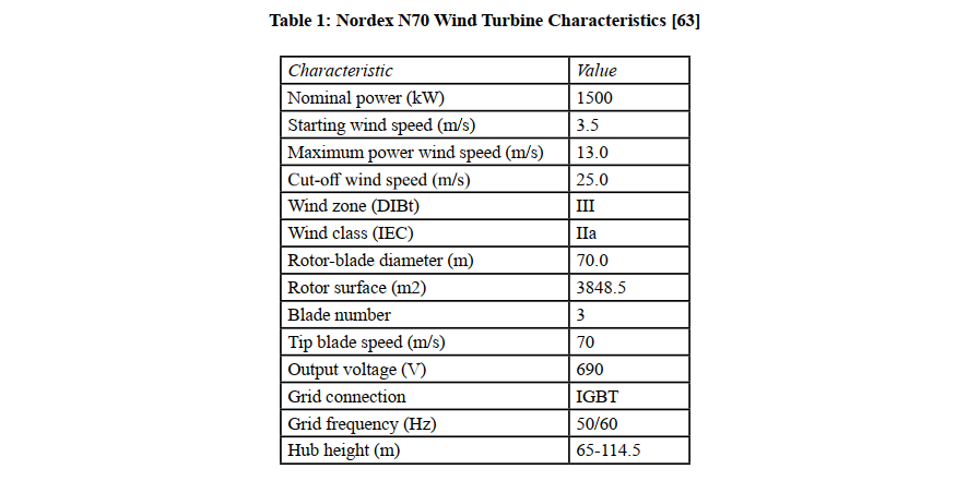
The wind farm comprises a group of wind turbines, Nordex N70, whose technical characteristics appear in Table 1.
 

We selected a hub height of 98 m, compatible with the following sites (Table 2)

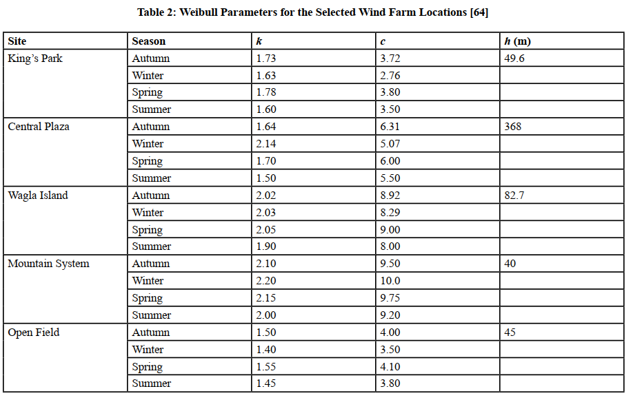
Based on the literature reference, we selected variable height and terrain type for the wind farm location [64]. Data for autumn and winter for King’s Park, Central Plaza, and Wagla Island correspond to the literature, while spring and summer values are derived from the calculation. We include two additional cases representing mountain and open field terrain so that we can diversify the wind farm selectable options.

The mountainous terrain is characterized by a higher k-value due to turbulences and erratic winds and a higher c-value because of higher wind speed at higher altitudes. We expect a lower k and c-value due to a more uniform wind flow in open-field terrain. Spring values tend to match autumn ones but are slightly higher because of the typical atmospheric variability in this season. In summer, the wind speed is more stable and tends to slow down, especially in areas far from the seaside or mountainous zones.

We calculate the wind speed at different heights using the classical expression [65]:
 

With α = 0.1748
The α-value corresponds to a moderate terrain rugosity and derives from statistical analysis of the selected wind farm location.

c) Fuel Cell System

The fuel cell system uses an electrolysis process to produce hydrogen in an electrolyze, storing the gas in a reservoir tank to feed the fuel cell. The electrolyze number and capacity determine the hydrogen production. Since the electrolyze operates at ambient pressure, we use a gas compressor to elevate the hydrogen pressure to the reservoir tank value.

Because the volumetric energy density of hydrogen is low, the tank pressure must be high, currently 350-700 bar; therefore, to avoid energy losses during gas compression, we use a three-stage compressor, reducing the pressure increase ratio at each stage and minimizing energy losses.

The fuel cell system uses PEM cells to facilitate a quick response in electricity demand from the external facility.

Simulation

A grid-connected facility may be considered a local autonomous installation where only the nearby energy generation and consumption matters. Previous studies prove the validity of the statement [66-67]. This configuration provides a frame to evaluate the energy balance in microgrids, allowing the optimization of the size and efficiency of a microgrid as a local system connected to the grid.

On the other hand, other studies emphasize that a non-connected microgrid may be used for energy balance optimization [68-69]. Using tools like HOMER, configurations can be evaluated based on local resource availability and consumption patterns. Nevertheless, a significant limitation derives from the inherent dependence on the grid for stability and backup power supply. Dynamic interactions like frequency regulation, voltage support, and emergency power supply are omitted, which are critical for the electric network stability when analyzing the microgrid independently from the grid. Therefore, the hypothesis should be established and the procedure validated by confronting the results with current world scenarios.

We apply the simulation to remote areas with no feasible or extremely costly grid connection, where the power supply depends on local energy resources and storage units, and to grid-integrated local zones where the principal power supply comes from renewable energy sources with the grid as a backup power system. Since the simulation considers the curtailment effect, storage energy units (BESS) or hybrid power generation systems are included in the study.

a) Energy Demand Curve Generation

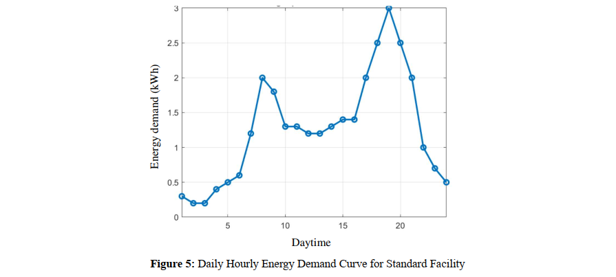
The energy demand curve is generated based on human patterns, divided into segments corresponding to different activity periods in a day. Figure 5 illustrates the energy demand curve for a standard facility.

The daily energy demand curve shows typical power peaks in the early morning and late afternoon, matching increases in human activity. Deviations from values shown in Figure 5 do not alter the simulation procedure, as the standard curve reflects an average behavior deviations from values shown in Figure 5 do not alter the simulation procedure.

 

b) Control System

The control system pursues the optimization of the energy distribution generated by multiple power sources. The protocol is relevant in scenarios where power generation exceeds energy demand, a more frequent situation due to the progressive implementation of autonomous renewable systems. The control system protocol aims at reducing energy losses and maximizing power management.

The protocol strategy is based on a dynamic evaluation of every power source's operating efficiency, determined by the energy losses to power generation ratio. Energy losses focus on the 

conversion process due to the voltage adjustment requirement and grid transportation, two critical factors in the efficiency determination. Therefore, the power source selection is based on power generation, energy efficiency, and availability. To this goal, the protocol continuously evaluates the energy losses, comparing values between the various power sources and classifying them according to power efficiency. This flexible process guarantees the selection of the most efficient power source at every moment, maximizing the energy supply and minimizing power losses.

When the energy balance is positive, the control system evaluates the efficiency of energy supply from every power source, Considering the output power and energy losses due to conversion and transportation, the control system receives information from the energy resource, solar radiation, wind speed, and hydrogen flow, calculating the available power generation from these resources using the corresponding equations described before. 

After determining the available power, the control system measures the input power from every source, solar, wind, and hydrogen, evaluating the efficiency by simply dividing input and available power, according to the expression.

Ρ_t is the power, with sub-index i accounting for the power source and super-indexes in and out for input and output.

Once all the power source's efficiency is determined, the control system compares the energy demand and the power generation from the most efficient power source. The control system blocks the power input from the other sources and limits the input power according to energy demand; if the balance is positive, the power generation is higher than the energy demand; if the balance is negative, the control system connects to the second most efficient power source and recalculates the energy balance, reducing the input power from the lowest efficiency power source, if necessary. The process repeats until all power sources are connected.

Simulation Results

The simulation runs on the following specific conditions:

• 60 MW solar thermal power plant, located 2 km away from the external facility
• 60 MW wind farm, with 40 wind turbines of 1.5 MW each, located 10 km away from the external facility
• 10 MW Fuel Cell system
• 50000 houses external facility

Figure 6 shows the daily hourly energy supply from every power source. It is noted that the fuel cell supplies constant power throughout the day because it does not depend on meteorological conditions like solar and wind power.

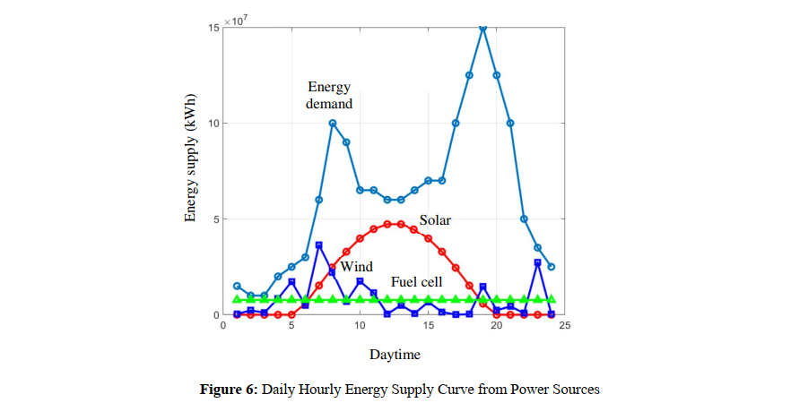
Solar power follows the conventional trend in a clear sky day with a maximum at midday and null contribution before sunrise and after sunset. Wind energy evolution follows a pattern defined by a statistical approach and is not representative of all possible conditions since the wind resource is random. If we add the three power source contributions, global power generation can be compared with the energy demand (Figure 7).

 

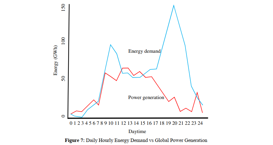
The control system intervenes when the energy balance is positive (power generation higher than energy demand), which occurs from 0 to 6 h and 12 to 15 h. In periods when the energy balance is null, the control system gives free access to all power sources since the combined energy supply from the three power sources equals the energy demand. In negative energy balance periods, the control system allows continuous energy supply from the power sources but opens the grid connection to compensate for the energy deficit. From midnight to early afternoon, 0 to 15 h, the global power generation covers the energy demand except in the period from 9 to 11 am, where an energy demand peak occurs. From 3 pm, the energy demand exceeds the global power generation, requiring grid energy supply to cover the deficit. We may solve the problem by enlarging the power source size, either solar, wind, fuel cell, or a combination of two or three; however, this solution increases the required land, the global investment, and the maintenance costs. Therefore, we accept a conservative configuration prioritizing economic reliability and energy efficiency. Enlarging the fuel cell system to cover the maximum energy unbalance at 20 h is not a good solution. It requires excessive oversizing due to the low fuel cell power contribution and the high energy unbalance. Using data from Figures 6 and 7, we obtain the following required fuel cell system enlargement:

F_sFC represents the enlargement size factor, ζ_D is the energy deficit, and ξ_FC is the fuel cell energy supply.

A similar situation occurs if an attempt is made to compensate for the energy unbalance at 8 am by enlarging the fuel cell system; in this case, the enlargement size factor is:

Analyzing the result from equation 16, it's concluded that enlarging the fuel cell system by a factor of 17.5 is nonsensical.

Which results in a too-high value. Therefore, the fuel cell system should remain at its present size, covering the energy deficit when solar and wind power are null or too low. Because the solar power plant supplies more energy in central day hours when the energy balance is positive, it is useless to enlarge it. The only remaining option is installing additional wind turbines to cover the energy deficit when necessary, connecting and disconnecting a variable number of turbines depending on the energy unbalance. In such a case, the additional wind turbine number should be:

This number is also nonsense. Therefore, the power system should remain unchanged because of the high energy deficit at 7 pm. Analyzing the evolution of global power generation and energy demand in Figure 7, we realize that in periods with an energy surplus, 0 to 6 am and 10 am to 2 pm, the control system should manage the power generation to make the energy balance null, connecting or disconnecting a power source or limiting the energy supply from the power source.

Control System

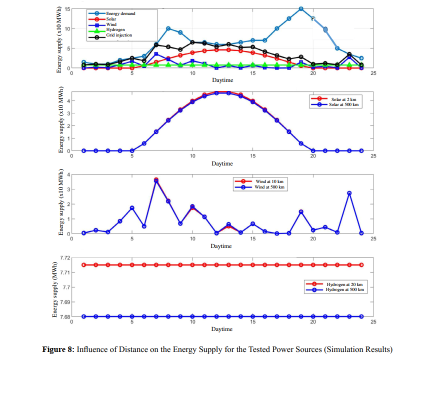
a) First case: Influence of Power Distance to External Facility
We tested various configurations to verify the power supply management reliability by the control system. To this goal, we evaluate the influence of distance from the power supply to the external facility, which modifies the energy losses during transportation and the input power.

Figure 8 shows the results for the first group of tests, considering an equal distance from any power source to the external facility equal to 500 km. The results show low or negligible influence, which proves that the control system model is efficient and accurate for transportation energy losses, minimizing the energy losses for long transmission distances.

 

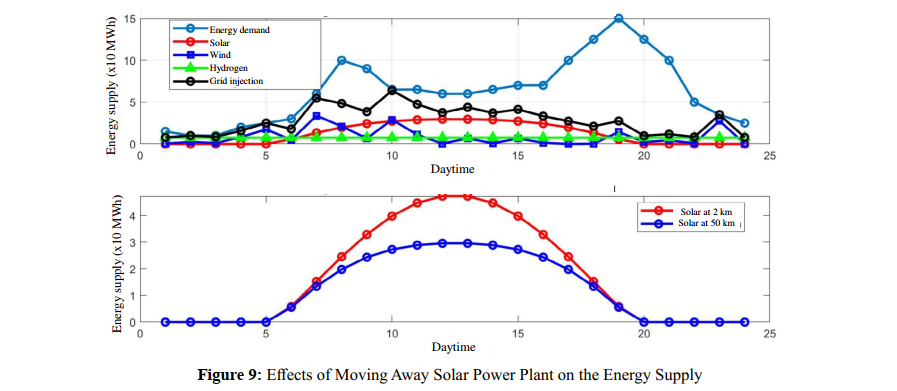
b) Second Case: Power Source Moving Away

The second type of test deals with the energy supply management from the power source or the grid. The goal is to evaluate whether or not it is suitable to import the energy from the grid instead of from the power source when the power plant moves away from its original site. In this second group of tests, we move the solar power plant 50 km from its original location, maintaining the wind farm and fuel cell system in its original site.

The simulation compares the energy supply using the grid or the power source. Figure 9 shows the simulation results for the solar power plant's energy supply.

When we move the solar power plant, the energy supply diminishes because of the higher distance; therefore, to compensate for the energy supply drop, we should use either the grid or any of the other two power sources, wind or hydrogen. Figure 10 shows the comparative results using power supply from the wind farm or the fuel cell system (distribution line) or importing energy from the grid (transmission line).

We realize that using the transmission line saves energy compared to the distribution line; the effect is more relevant for the fuel cell system, which operates at constant power supply. In the wind farm case, the difference is negligible except at 10 am, which matches the first daily energy unbalance peak.

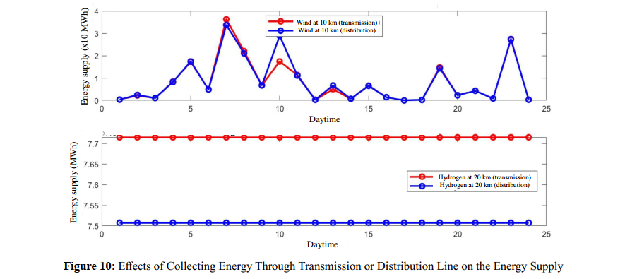
This result is coherent with current practice since the distribution lines are designed for a short-distance power supply. The transmission lines operate better at high distances because of the higher transportation voltage.

Analyzing results from this second group of tests, we observe that the distribution lines operate with lower efficiency if any power source moves away from its original site. In the case of an energy supply drop in the solar power plant caused by a longer distance to the external facility, the control system commutes to the wind farm power supply since it operates at equal efficiency to the grid power supply. The fuel cell works at a lower efficiency than the grid.

Repeating the process for the wind farm, moving away from 10 to 50 km, we obtain the following results (Figure 11):
 

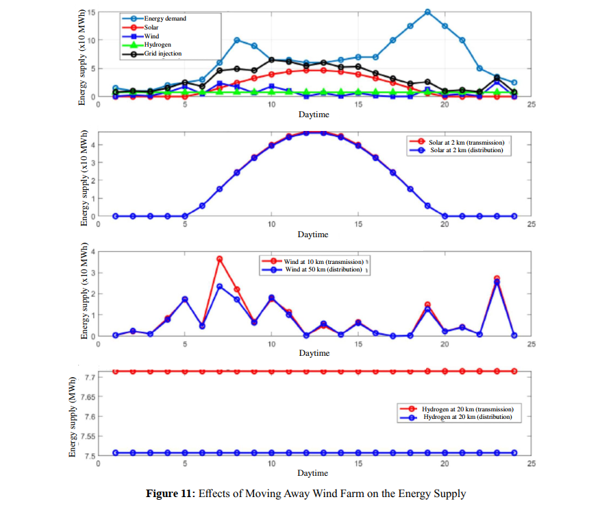
We observe that transmission supplies a little more energy than distribution for the wind farm due to the longer distance when we move the power source to 50 km away. Solar plant power supply remains unaltered. The efficiency of using the fuel cell system is lower than taking energy from the grid; therefore, in this case, the control system commutes to the solar power plant for extra energy when needed, leaving the fuel cell as a reservoir power source. Now, moving the fuel cell system from 20 to 50 km, we have (Figure 12):

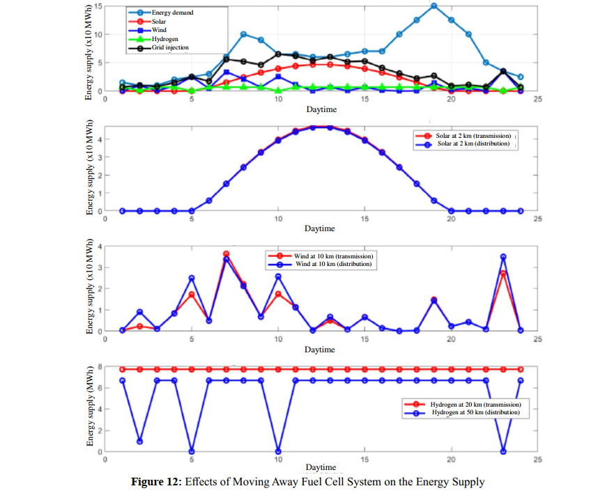
We notice that solar and wind power source supplies remain unaltered. In the present case, the control system reduces the hydrogen flow, lowering the fuel cell power supply to compensate for the increase in wind farm power supply. This situation proves the control system's reliability and the validity of the proposed protocol.

c) Third Case: Energy Demand Reduction

The third simulation tests group consists of reducing the energy demand to evaluate the influence on the power system performance and how the control system reacts to this event.

Figure 13 shows the simulation results for an energy reduction to

 

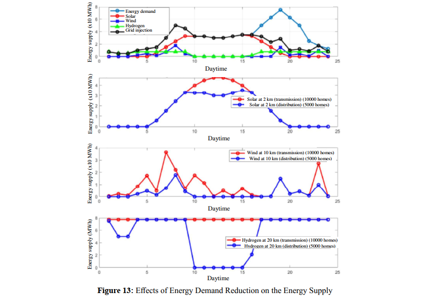
Reducing demand by half produces interesting cases of reduction in all technologies. We see that solar does not supply all it can when the sun is closer to the perpendicular since there is no demand. In the same way, wind power is the last one selected by the controller, and we see that it has high levels of reduction, making this source highly inefficient. The same occurs with hydrogen. In this scenario, it is clear that we need to implement BESS systems so there is no excess energy-wasting, supplying power in the hours when generation is not meeting demand, from 5 p.m. until the end of the days.

d) Fourth Case: Variation of Power Generation

In the fourth group of tests, we modify the power generation, either increasing or decreasing it. We consider the following situations:
*Solar power plant generation cut down by half In this situation the results are (Figure 14):

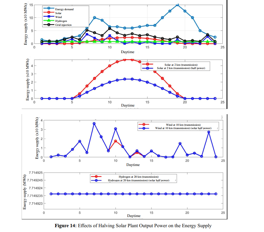
As the nominal power of the solar park decreases, since it is the source that the controller selects first, the rest of the sources that did not give their maximum are forced to give their maximum, like the wind power, which has to try to make up for what solar power was giving; therefore, we can inject more. There is less reduction for this source. In this scenario, any technology type is applicable.

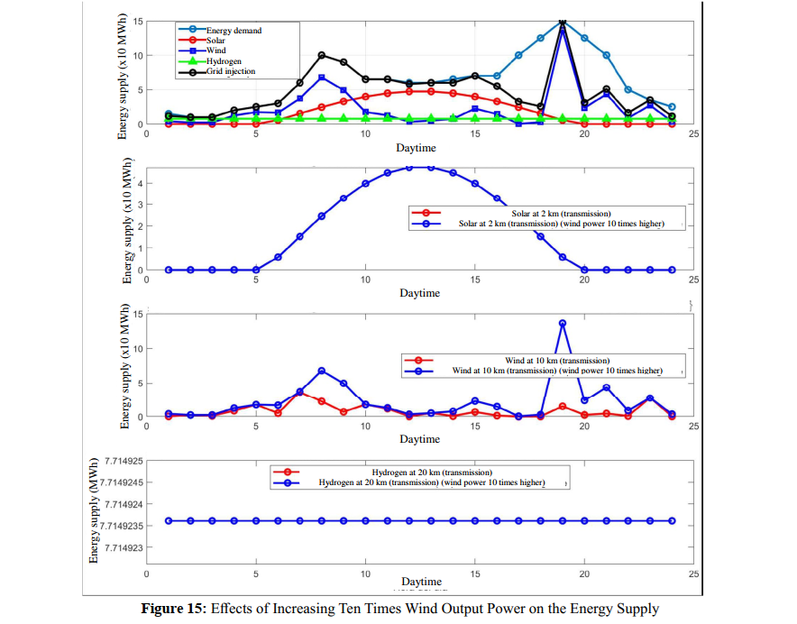
* Wind power increased ten times

Applying this condition, the simulation produces the following results (Figure 15) :

If we increase the nominal power of the wind farm, this power source is the last to come into play, providing more energy when there is more demand than what solar and hydrogen can provide. As we said before, installing wind farms in the area is a good option since there is a low energy reduction. This configuration shows that we can simulate the park that we want to install in an area and see if it will have a reduction or not.

 

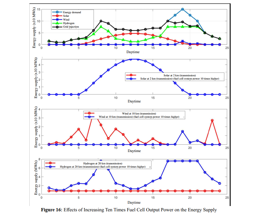
* Fuel cell power increased ten times

This new configuration produces the following results (Figure 16)
If we increase the fuel cell output power ten times, wind power does not participate because it generates a very high energy reduction. Therefore, it is not advisable to install more wind turbines unless their electric energy losses are lower than those of the fuel cell  unit. We observe that the fuel cell power generation suffers a high reduction, especially during low-demand periods and in high solar generation time. Therefore, for the fuel cell power system, it would be interesting to install a Battery Energy Storage System (BESS) to store the energy excess and release it during times of greater demand. The same consideration applies to the wind resource.

 

e) Change of Location and Season

In all previous cases, the location for solar and wind resources is Kings Park in autumn. For the new simulation, the location is changed to Wagla Island in springtime. The change in location and season produces variations in natural resources like solar and wind power, which depend on climatic and meteorological conditions. Wagla Island, in springtime, has higher wind power but a smaller solar resource. Fuel cell output power does not alter because it is independent of climatic and meteorological conditions.

The new simulation looks for evaluating the influence of simultaneous changes in two power sources, regarding previous analysis where only one power source modifies. In the proposed configuration, with only two power sources depending on climatic and meteorological conditions, only one case arises; nevertheless, the study can be extended to other configurations where three or more power sources intervene, all of them depending on environmental conditions. In such a case, the analysis should be extended to additional options, but the procedure remains.

Figure 17 shows the simulation results.

We see that solar, the one with the lowest electrical losses in our model, is the first selected. However, we obtain less energy with the same nominal power. In the same way, we obtain much more energy with the same nominal power from the wind farm since the wind turbines can obtain more energy from the wind. This situation occurs in the afternoon with a higher energy demand than consumption. Thus, we see that the model works correctly in different locations. For the first time, the consumption and the demand curve are equal for almost all hours.

f) Change of Altitude

The last simulation focuses on an altitude change to evaluate the influence of atmospheric conditions on environment-dependent natural resources like solar and wind, especially the last one.

To this goal, we have designed an imaginary scenario in a mountainous region at a specific altitude of 2000 m above sea level. The altitude value is not critical since the effect on the power generation and energy supply follows the same trend as in the present study.

Figure 18 shows the simulation results for this case.

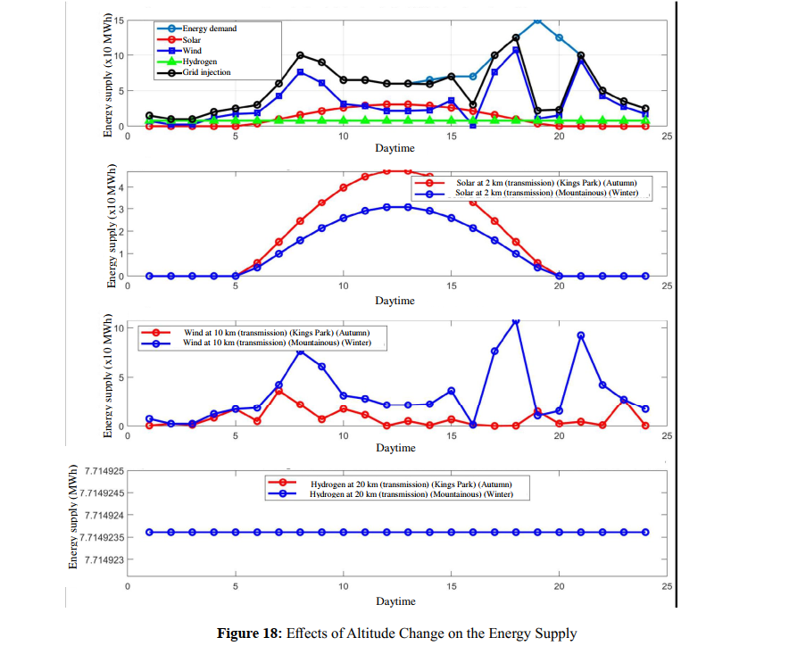
Now, moving to an invented mountain system in winter, with lower solar resources and high wind power, similarities with the previous case can be noted. Although the wind provides high power, its intermittency and randomness mean that the required wind energy cannot be fully utilized during peak consumption hours (7-8 pm), leading to financial losses. Therefore, a Battery Energy Storage System (BESS) is of interest to compensate for the wind resource intermittency.

Conclusions

This work demonstrates the feasibility of integrating multiple renewable energy sources, such as solar, wind, and hydrogen, in local networks. The complementarity of power source combinations helps mitigate the inherent limitations of each source, such as intermittency and variability, resulting in a more stable and reliable power supply. This approach enhances local network energy security and strengthens the energy grid's capacity to respond to energy demand fluctuations.

The proposed control system optimizes different power sources, considering critical factors like energy demand, conversion efficiency, and energy losses associated with each power technology. This optimization leads to significant energy efficiency improvements, minimizing carbon emissions, and contributing to global sustainability goals.

The simulation results analysis validates the protocol, aligning with testing results under current operating conditions. The developed methodology enables the selection of suitable renewable energy configurations for specific local conditions. Simulated tests in variable scenarios demonstrate the procedure's versatility, highlighting its ability to adapt to variable energy demand and operating conditions.

Flexibility and adaptation capacity are key methodological characteristics, allowing for multiple power source combinations, which are particularly relevant in a world of continuous innovation, implementation, and technological changes. The application of the proposed methodology improves energy efficiency and sustainability.

Finally, the proposed system protects the environment since it contributes to reducing carbon emissions and promotes a more sustainable energy model. The methodology applies to variable power system scales and geographic locations, reinforcing its
validity and potentiality for application in a transition process toward a cleaner and more resilient energy system.
 

References

1. Dong, K., Hochman, G., Zhang, Y., Sun, R., Li, H., & Liao, H. (2018). CO2 emissions, economic and population growth, and renewable energy: empirical evidence across regions. Energy Economics, 75, 180-192.
2. Al-Badi, A., & AlMubarak, I. (2ues019). Growing energy demand in the GCC countries. Arab Journal of Basic and Applied Sciences, 26(1), 488-496.
3. Khan, I., Hou, F., & Le, H. P. (2021). The impact of natural resources, energy consumption, and population growth on environmental quality: Fresh evidence from the United States of America. Science of the Total Environment, 754, 142222.
4. Dincer, I., & Rosen, M. A. (1999). Energy, environment and sustainable development. Applied energy, 64(1-4), 427-440.
5. Hubbert, M. K. (1949). Energy from fossil fuels. Science, 109(2823), 103-109.
6. Ghosh, S. K., & Ghosh, B. K. (2020). Fossil fuel consumption trend and global warming scenario: Energy overview. Glob. J. Eng. Sci, 5(2), 1-6.
7. Pirani, S. (2018). Burning up: A global history of fossil fuel consumption. Pluto Press.
8. Johnson, B. (2017). Carbon nation: Fossil fuels in the making of American culture. University Press of Kansas.
9. Högselius, P. (2023). The political history of fossil fuels: coal, oil, and natural gas in global perspective. In Handbook on the Geopolitics of the Energy Transition (pp. 67-83). Edward Elgar Publishing.
10. Balat, M. M. Y. C. (2007). Status of fossil energy resources: A global perspective. Energy Sources, Part B: Economics, Planning, and Policy, 2(1), 31-47.
11. Keeling, C. D. (1973). Industrial production of carbon dioxide from fossil fuels and limestone. Tellus, 25(2), 174-198.
12. Bos, K., & Gupta, J. (2018). Climate change: the risks of stranded fossil fuel assets and resources to the developing world. Third World Quarterly, 39(3), 436-453.
13. Soeder, D. J., & Soeder, D. J. (2021). Fossil fuels and climate change. Fracking and the Environment: A scientific assessment of the environmental risks from hydraulic fracturing and fossil fuels, 155-185.
14. Shanmugam, G. (2023). Fossil fuels, climate change, and the vital role of CO2 to people and plants on planet Earth. Bulletin of the Mineral Research and Exploration, 1(early view), 1-1.
15. Höök, M., & Tang, X. (2013). Depletion of fossil fuels and anthropogenic climate change—A review. Energy policy, 52, 797-809.
16. Hoel, M., & Kverndokk, S. (1996). Depletion of fossil fuels and the impacts of global warming. Resource and energy economics, 18(2), 115-136.
17. Shafiee, S., & Topal, E. (2008). An overview of fossil fuel reserve depletion time. In 31st IAEE International Conference, Istanbul pp. 18-20.
18. Mohr, S. H., Wang, J., Ellem, G., Ward, J., & Giurco, D. (2015). Projection of world fossil fuels by country. Fuel, 141, 120-135.
19. Solomon, B. D., & Krishna, K. (2011). The coming sustainable energy transition: History, strategies, and outlook. Energy Policy, 39(11), 7422-7431.
20. Leach, G. (1992). The energy transition. Energy policy, 20(2), 116-123.
21. Petit, V. (2017). Energy transition. Springer International Publishing AG.
22. Lowitzsch, J., Lowitzsch, S., & Sangster, E. T. (2cap19). Energy transition. Springer International Publishing.
23. Luthra, S., Kumar, S., Garg, D., & Haleem, A. (2015). Barriers to renewable/sustainable energy technologies adoption: Indian perspective. Renewable and sustainable energy reviews, 41, 762-776.
24. Gowrisankaran, G., Reynolds, S. S., & Samano, M. (2016). Intermittency and the value of renewable energy. Journal of Political Economy, 124(4), 1187-1234.
25. Kosonen, I. (2018). Intermittency of renewable energy; review of current solutions and their sufficiency.
26. Sovacool, B. K. (2009). Rejecting renewables: The socio-technical impediments to renewable electricity in the United States. Energy policy, 37(11), 4500-4513.
27. Boghdady, T. A., Alajmi, S. N., Darwish, W. M. K., Hassan, M. M., & Seif, A. M. (2021). A Proposed Strategy to Solve the Intermittency Problem in Renewable Energy Systems Using A Hybrid Energy Storage System. WSEAS Transactions on Power Systems, 16(2021), 41-51.
28. Bremen, L. V. (2010). Large-scale variability of weather dependent renewable energy sources. In Management of weather and climate risk in the energy industry (pp. 189-206). Springer Netherlands.
29. Roy, P., He, J., Zhao, T., & Singh, Y. V. (2022). Recent advances of wind-solar hybrid renewable energy systems for power generation: A review. IEEE Open Journal of the Industrial Electronics Society, 3, 81-104.
30. Shrivastwa, R. R., Hably, A., Bacha, S., Mesnage, H., & Guillaume, R. (2ues for Ancillary Service. In 2020 IEEE International Conference on Industrial Technology (ICIT) (pp. 536-541). IEEE.
31. Nehrir, M. H., Wang, C., Strunz, K., Aki, H., Ramakumar, R., Bing, J., ... & Salameh, Z. (2011). A review of hybrid renewable/alternative energy systems for electric power generation: Configurations, control, and applications. IEEE transactions on sustainable energy, 2(4), 392-403.
32. Atawi, I. E., Al-Shetwi, A. Q., Magableh, A. M., & Albalawi, O. H. (2022). Recent advances in hybrid energy storage system integrated renewable power generation: Configuration, control, applications, and future directions. Batteries, 9(1), 29.
33. Sinha, S., & Chandel, S. S. (2014). Review of software tools for hybrid renewable energy systems. Renewable and sustainable energy reviews, 32, 192-205.
34. Lund, H., & Mathiesen, B. V. (2009). Energy system analysis of 100% renewable energy systems—The case of Denmark in years 2030 and 2050. Energy, 34(5), 524-531.
35. Duffie, J. A., Beckman, W. A., & Blair, N. (2020). Solar engineering of thermal processes, photovoltaics and wind. John Wiley & Sons.
36. Johnson, F. S. (1954). The solar constant. Journal of Atmospheric Sciences, 11(6), 431-439.
37. Eltbaakh, Y. A., Ruslan, M. H., Alghoul, M. A., Othman, M. Y., & Sopian, K. (2012). Issues concerning atmospheric turbidity indices. Renewable and Sustainable Energy Reviews, 16(8), 6285-6294.
38. Rele, B., Hogan, C., Kandanaarachchi, S., & Leigh, C. (2023). Short-term prediction of stream turbidity using surrogate data and a meta-model approach: A case study. Hydrological Processes, 37(4), e14857.
39. Javanshir, A., & Sarunac, N. (2017). Thermodynamic analysis of a simple Organic Rankine Cycle. Energy, 118, 85-96.
40. Yamamoto, T., Furuhata, T., Arai, N., & Mori, K. (2001). Design and testing of the organic Rankine cycle. Energy, 26(3), 239-251.
41. Van Hemelrijck, E. (1983). The oblateness effect on the extraterrestrial solar radiation. Solar Energy, 31(2), 223-228.
42. Wang, L., Chen, Y., Niu, Y., Salazar, G. A., & Gong, W. (2017). Analysis of atmospheric turbidity in clear skies at Wuhan, Central China. Journal of Earth Science, 28, 729-738.
43. Lucía Serrano Gallar (2015) Modelling and Simulation of Solar Field Configuration for Solar Thermal Tower Power Plants: Influence of Concentrator Optics on Energy Generation. Doctoral Thesis. Complutense University of Madrid.
44. Raj, M., & Bhattacharya, J. (2023). Precise and fast spillage estimation for a central receiver tower based solar plant. Solar Energy, 265, 112103.
45. Burton, T., Sharpe, D., Jenkins, N., & Bossanyi, E. (2009). Wind Characteristics and Resources. In \textit{Wind Energy Explained} (Chapter 2, pp. 23-89). John Wiley & Sons. https://doi.org/10.1002/9781119994367.ch2
46. Sarkar, A., & Behera, D. K. (2012). Wind turbine blade efficiency and power calculation with electrical analogy. International Journal of Scientific and Research Publications, 2(2), 1-5.
47. Sequeira, C., Pacheco, A., Galego, P., & Gorbeña, E. (2019). Analysis of the efficiency of wind turbine gearboxes using the temperature variable. Renewable Energy, 135, 465-472.
48. Weibull, W. (1951). A statistical distribution function of wide applicability. Journal of applied mechanics.
49. Manwell, J. F., McGowan, J. G., & Rogers, A. L. (2010). Wind energy explained: theory, design and application. John Wiley & Sons.
50. Cheekatamarla, P. K., & Finnerty, C. M. (2006). Reforming catalysts for hydrogen generation in fuel cell applications. Journal of Power Sources, 160(1), 490-499.
51. Damle, A. S. (2009). Hydrogen production by reforming of liquid hydrocarbons in a membrane reactor for portable power generation—Experimental studies. Journal of Power Sources, 186(1), 167-177.
52. Dicks, A. L. (1996). Hydrogen generation from natural gas for the fuel cell systems of tomorrow. Journal of power sources, 61(1-2), 113-124.
53. Okere, C. J., & Sheng, J. J. (2023). Review on clean hydrogen generation from petroleum reservoirs: Fundamentals, mechanisms, and field applications. International Journal of Hydrogen Energy.
54. Iulianelli, A., Ribeirinha, P., Mendes, A., & Basile, A. (2014). Methanol steam reforming for hydrogen generation via conventional and membrane reactors: A review. Renewable and Sustainable Energy Reviews, 29, 355-368.
55. Agrell, J., Lindström, B. A. É. R. D., Pettersson, L. J., & Järås, S. G. (2002). Catalytic hydrogen generation from methanol. Catalysis-Specialist Periodical Reports, 16, 67-132.
56. StojiÄ?, D. L., Marčeta, M. P., Sovilj, S. P., & MiljaniÄ?, Š. S. (2003). Hydrogen generation from water electrolysis— possibilities of energy saving. Journal of power sources, 118(1-2), 315-319.
57. Naimi, Y., & Antar, A. (2018). Hydrogen generation by water electrolysis. Advances in hydrogen generation technologies, 1.
58. Suleman, F., Dincer, I., & Agelin-Chaab, M. (2015). Environmental impact assessment and comparison of some hydrogen production options. International journal of hydrogen energy, 40(21), 6976-6987.
59. Zhan, T., Bie, R., Shen, Q., Lin, L., Wu, A., & Dong, P. (2020, November). Application of electrolysis water hydrogen production in the field of renewable energy power generation. In IOP Conference Series: Earth and Environmental Science (Vol. 598, No. 1, p. 012088). IOP Publishing.
60. Lehner, M., Tichler, R., Steinmüller, H., & Koppe, M. (2014). Power-to-gas: technology and business models (pp. 7-17). Cham: Springer International Publishing.
61. Larminie, J., & Dicks, A. (2003). Fuel Cell Systems Explained. John Wiley & Sons.
62. Ewan, B. C. R., & Allen, R. W. K. (2005). A figure of merit assessment of the routes to hydrogen. International Journal of Hydrogen Energy, 30(8), 809-819.
63. https://es.wind-turbine-models.com/turbines/519-nordex-n70
64. Lun, I. Y., & Lam, J. C. (2000). A study of Weibull parameters using long-term wind observations. Renewable energy, 20(2), 145-153.
65. Fox, R. W., McDonald, A. T., Pritchard, P. J. (2011). Introduction to Fluid Mechanics (8th ed.). John Wiley Sons.
66. Adaramola, M. S., Agelin-Chaab, M., & Paul, S. S. (2014). Analysis of hybrid energy systems for application in southern Ghana. Energy Conversion and Management, 88, 284-295.
67. Algarni, S., Muhsen, N., Etemadi, A. H. (2020). "Optimal sizing and operation of hybrid renewable energy systems considering uncertainties". Renewable Energy, 145, 1128- 1143.
68. Bukar, A. L., Tan, C. W., Ayop, S. (2019). "A review of optimization techniques for sizing hybrid renewable energy systems". Sustainable Cities and Society, 49, 101634.
69. Carballo, J., Hernández, J. C., Jordá, L. (2021). “Optimización de sistemas híbridos renovables con herramientas de simulación”. Energías Renovables y Medio Ambiente, 28(2),45-59.

70. HOMER Software. HOMER Energy is now UL Solutions. HOMER - Hybrid Renewable and Distributed Generation System Design Software (homerenergy.com)

71. Oxford Academic. (2021). “Dynamic interactions in power systems with high renewable energy penetration”. International Journal of Electrical Power Energy Systems, 131, 107077.