A Deep Learning Prototype Tested Against 2nd Order Statistical Central Composite Design (CCD) Models

Introduction

Data Science and its related models has had tremendous applications this decade, speeding up various applications in design, engineering, manufacturing and Research and Development (R & D) processes. This rapidly emerging field of knowledge coupled with Artificial Intelligence (AI) and Machine Learning (ML) enables engineers and scientists to develop more robust design of experiments and triggers an innovative surge in more reliable design and analysis. While data science deals with analysis and visualization which are key to making sense of data, the fundamental challenge for all engineers, scientists and managers is building an infrastructure capable of collecting and processing data from a variety of sources. Data Science, Machine Learning and AI are a must for the contemporary researchers to make meaningful innovations. Through generating intelligence, accelerating innovation and fully enabling mobility, data science professionals can remove barriers to adoption, improve efficiencies, mitigate risk and look forward to improved productivity. Traditionally, we were designing to sequentially process data and to use specific program code instructions in the processing. Deep learning (DL) which is a subset of Machine Learning allows computer systems to analyze data to provide insights and predictions about the data. Machine learning refers to any type of computer program that can learn by itself without being programmed by a human. Deep learning, also known as deep structured learning that uses artificial neural networks. Deep learning systems can be supervised, partially supervised or unsupervised. This effort often starts with improving data storage and retrieval, enabling better utilization of data to improve service levels and thereby competitive and comparative advantages.

Problem Background

(Statistical Models derived from CCD Experiments formed the basis for evaluating DL)

The central composite design (CCD) is the most commonly used fractional factorial design used in the response surface model. In this design, the center points are augmented with a group of axial points called star points. With this design, attempts are made to estimate quickly the first-order and second-order terms. While our more than forty years of experience with statistical process modeling and optimization have been valuable, we believe that deep learning (DL), an emerging aspect of machine learning and artificial intelligence, can produce even better results than traditional mathematical and statistical techniques, including response surface methodology (RSM) [1]. The two key applications of artificial neural networks are found in classification, and regression [2]. In the later, DL's ability to accurately represent complex non-linear multivariable relationships between process control (input) factors and response (output) variables has shown promise, where the basic modeling theory based on scientific principles and laws is unavailable. Furthermore, quadratic second-order response functions, which are commonly used to build empirical process models, may not be flexible enough to capture complex non-linear relationships, making DL a more suitable approach for these cases [2]. The success of machine learning in combination with evolutionary optimization genetic algorithm (GA) in optimizing discontinuous functions further highlights the potential of DL in complex modeling problems [3]. A very significant application modeling processes by neural nets is in optimization, an area in which the problems that must be optimized are not linear or polynomial; they cannot be precisely resolved, and they must be approximated [4].

To test the claims of DL's superior modeling capability, it is attempted here in this paper to build a compact DL model by using Tensorflow. In the field of engineering and scientific processes where theory is not yet sufficiently advanced, the commonly used statistical process engineering methodology is the central composite experimental design (CCD), which involves a series of planned experiments with prescribed input variable levels and observed response data [3]. CCD is useful for studying non-linear response surfaces or significant low-order interactions among input variables. However, its mathematical complexity limits its ability to study only up to second-order effects, potentially missing out on higher order non-linearities present in the process. DL, on the other hand, can learn these non linearities through its modeling parameters updated from sample input-response data presented during training. DL models use multiple computational layers and advanced techniques such as convolutional neural networks (CNN) to extend their predictive capability in object detection, voice and image classification, and segmentation. These artifacts, now common in our physical world, such as self-driving cars and language modeling, can handle a significant degree of non-linearity. Therefore, we believe that incorporating DL into the study of input-response relationships in engineering and scientific processes, in conjunction with traditional statistical methods, can provide a more comprehensive understanding of complex systems.

To objectively compare the efficacy of deep learning (DL) and response surface methodology (RSM) in data-based process modeling, we undertook and utilized a standard problem from the well-respected and widely followed textbook, "Design and Analysis of Statistical Experiments" [3]. The problem involve modeling a chemical process using Center Composite Experimental Design (CCD) to produce a second-order regression model with two input variables and three responses, with its complete statistical analysis provided in the text. This provided a baseline for comparison with a DL-based prediction model we developed using the same data [5]. The DL model was hyperparameter tuned using guidance from current literature and showed excellent performance, closely matching the results from the text. In fact, in several examples, the DL model yielded smaller root mean square errors. This experience is becoming increasingly common for machine learning and DL investigators [1,6]. Therefore, incorporating DL in process studies with suitably collected input data before invoking RSM could lead to more accurate results. The Python/Tensorflow code for the DL model used in this study is enclosed in the Appendix.

Montgomerys Second-Order Chemical Process Model

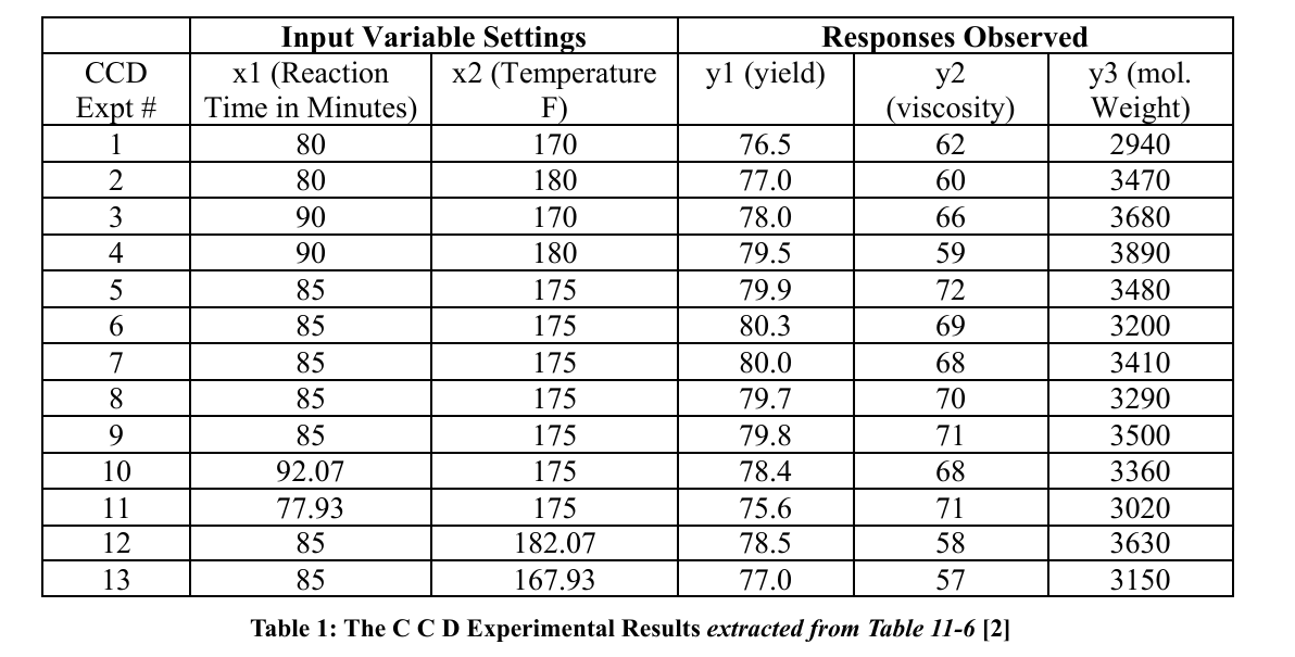
The current state-of-the-art approach to empirically model multi-factor processes and optimize them is clearly explained in [3]. In this study, a chemical process was investigated by manipulating two operating conditions, reaction time (x1) and reaction temperature (x2), following the central composite design (CCD) experimental scheme. The responses observed in each experiment were yield (y1), viscosity (y2), and molecular weight (y3) (see Table 1). According to this design allows the development of second-order response models in x1 and x2, enabling the optimization of responses y1, y2, and y3 when required [3]. Although we do not follow the optimization steps outlined in, we quote the multi-regression prediction model for yield (y1) to which DL would be compared, using the relevant data from Table 1 [3].

The author of obtained the 2nd order regression model for yield (y1) as follows:
Yield (y1) = -1430.52285 + 7.80749 Time + 13.27053 Temp - 0.055050 Time²- 0.0400050 Temp2 + 0.010000 Time Temp (1)
We used the model presented in (1) to compare its predictions with the DL models we subsequently built. Reference (Montgomery, 2001) provides two more regression models built using the data of Table 1, as follows.
Viscosity (y2) = -9030.74 + 13.393 Time + 97.708 Temp - 2.75×0.01 Time² - 0.26757 Temp² - 5×0.01 Time Temp..... (2)
Molecular Weight (y3) = -6308.8 + 41.025 Time + 35.473 Temp ...............  (3)

Note that each of these process models (1), (2) and (3) are at best second order regression models. The CCD scheme for conducting the experiments would not yield any information about higher order effects or interactions. However, nature’s acts are not restricted to second order effects only. Such higher order interactions and effects cannot be explored by CCD. Even in Resolution V experimental designs two-factor interactions are aliased with three-factor interactions [3]. Such occurrences seriously affect experimental investigation of complex factor effects and their interactions.

Process Model Building by Deep Learning (DL)

What follows is a brief outline of the DL model building procedure. For more details, we refer the reader to citations [7,2]. DL is a machine learning algorithm that utilizes artificial neural networks with multiple layers capable of learning a wide range of computational tasks through modifiable parameters. After setting up the network architecture, DL is trained to adjust its weights, minimizing the difference between predicted and actual output. This training process involves exposing the algorithm to a large amount of labeled data to optimize the interconnecting weights in the network. The complexity and accuracy of DL’s performance increase with the number of layers [8]. This feature is heavily utilized in tasks like speech and image recognition, natural language processing, and decision making. However, added complexity also affects DL efficiency [9]. Efforts are being continually made to develop tools and frameworks such as TensorFlow, PyTorch, and Keras to enhance DL efficiency. These developments have significantly benefited industries like healthcare, transportation, and finance, among many others. DL is efficient and improves predictive accuracy compared to simple ANNs. Building a DL model is a systematic process that involves several steps. Firstly, the problem needs to be defined and relevant data needs to be gathered. In our case, we aimed to create a DL model that would emulate the statistical CCD/ RSM method to determine input-response relationships within a suitably collected dataset, as demonstrated in Table 11-3 of [3].

The next step is to preprocess the data to ensure its compatibility with the desired format. In our case, we strictly followed the Python and TensorFlow coding conventions (as shown in the Appendix), which can be seen in the code under the section # Set up the input data. Once the data is preprocessed, the network architecture needs to be specified. For the DL model, a flow forward layout with two input nodes to receive the input, and a hidden layer that was specified was used. This aspect of the model can be empirically optimized to ensure the DL's efficient and accurate performance, as shown in the code under the section # Define the model architecture. After selecting the appropriate architecture, there were options to build the model using a deep learning framework, such as TensorFlow, PyTorch, or Keras. In this case, TensorFlow, Keras, and numpy were chosen to define the layers of the model, connect them, and set the hyperparameters like learning rate and batch size. Next, the model was compiled and specified the performance metric as the mean squared error between the observed response and the DL's predicted response for the same experimental factor setting (x1 and x2 in Table 1). To train the model, it was provided with pairwise x (input data), y (corresponding output or response data), and the epoch number to control the model's convergence iterations. The connecting weights between the layers of the model were optimized using the ADAM optimizer, a global optima-seeking numerical heuristic.

Once the model was trained, the researchers were ready to predict the output for new data and evaluate its performance. However, due to the limited availability of experimental data dictated by Table 11-6, they used all 13 data points for training and performance evaluation. As a result, their ability to validate the model's generalization performance to new data was limited. Access to the process engineering setup that generated Table 11-6 was impossible, making the partitioning of the small amount of available data into train/evaluate subsets impractical for the sake of precision. Therefore, while evaluation of the model's performance using separate test data is integral to building a DL model, in this exercise, it was not feasible. Nonetheless, their reason for reusing the data from Table 11-6 was compelling, given the circumstances. Evaluating a DL model involves fine-tuning its hyperparameters, which can significantly impact the quality and performance of the model in production. The hyperparameters include the learning rate, regularization strength, number of hidden layers, number of nodes in each layer, and batch size. Although there are some suggested guidelines for training these hyperparameters, they are generally domain-specific and may require modifications to the model's architecture. To address this, the researchers used the grid search method to find the optimal hyperparameters for their model.

However, even with the optimal hyperparameters, there are still challenges in achieving convergence without overtraining the model. One issue we encountered was setting the random seed, which determines the computational path taken by the heuristic global optimization. We conducted multiple trials with different seeds and epochs to heuristically attain convergence while avoiding overtraining. These challenges highlight the importance of careful and iterative testing and optimization of the DL model.

Comparison of CCD Results and DL Predictions

In order to compare the predictability performance of CCD experiments and DL, we utilized the standard problem presented in Chapter 11 of [3]. The DL's model training and validation data were extracted from Table 11-6 of, which provided us with a reliable dataset for our analysis [3]. To supplement this data, we also used Table 1 of this paper, which displays the relevant CCD experimental input and response data for yield, viscosity, and molecular weight observed in the real chemical process. By utilizing these data sources, we were able to conduct a comprehensive analysis and compare the efficacy of CCD and DL for modeling multi-factor processes.

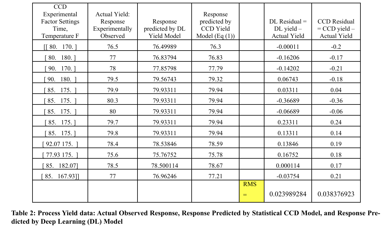
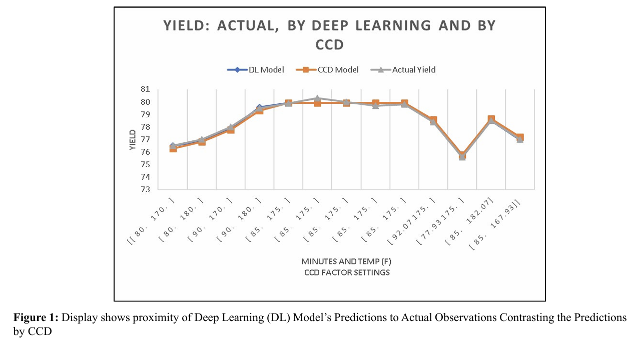
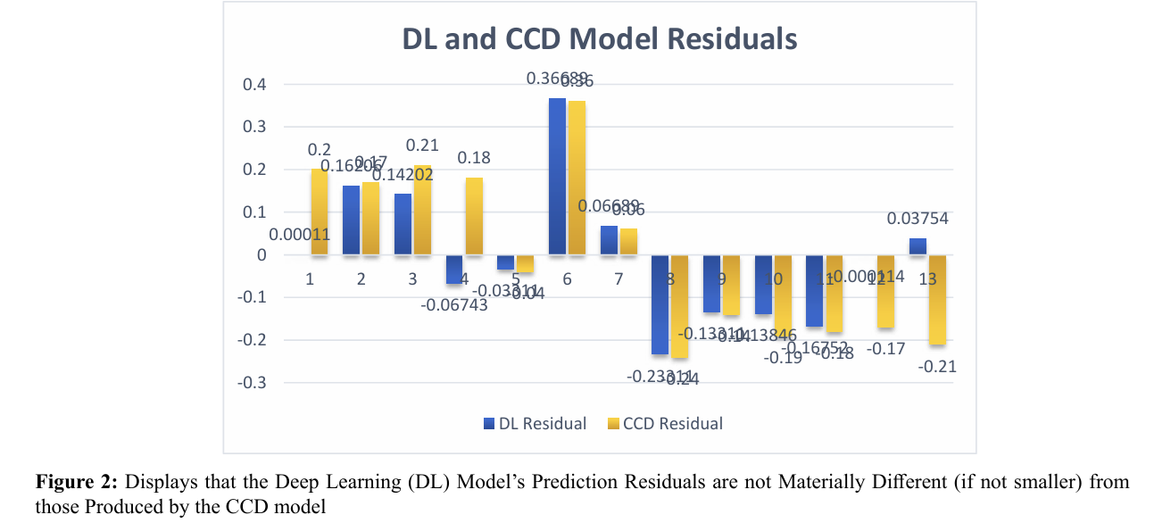
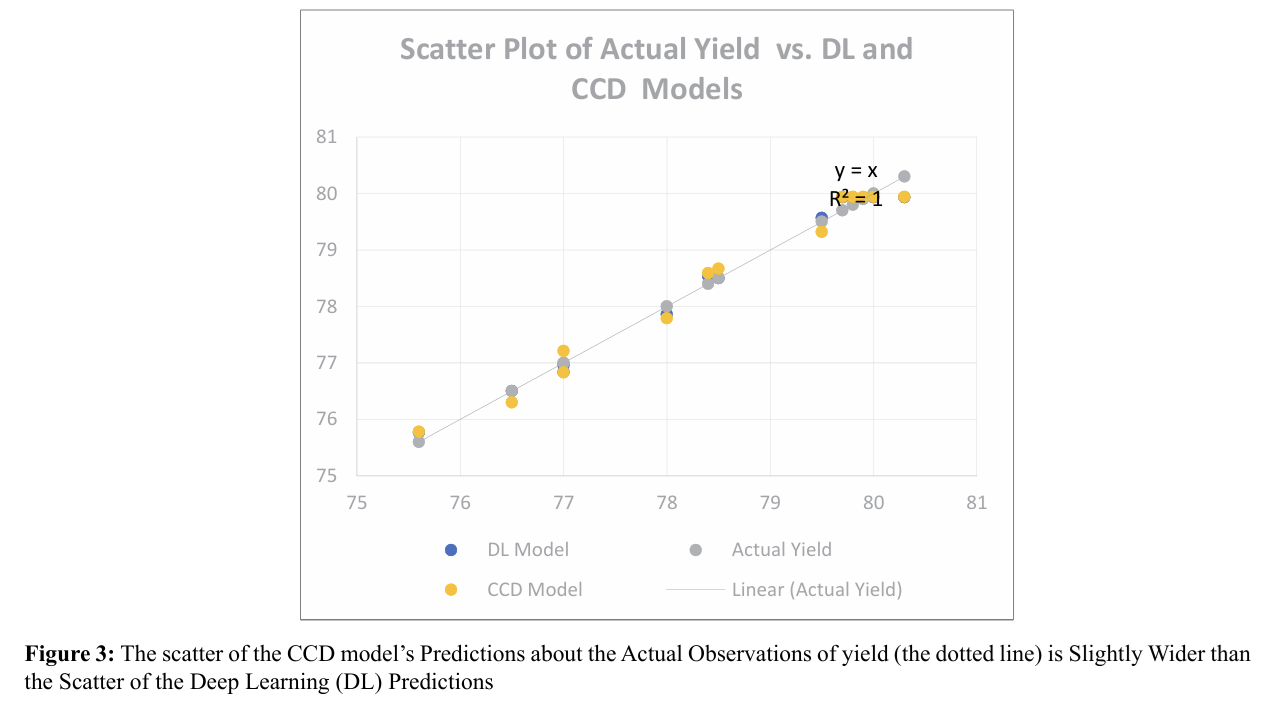
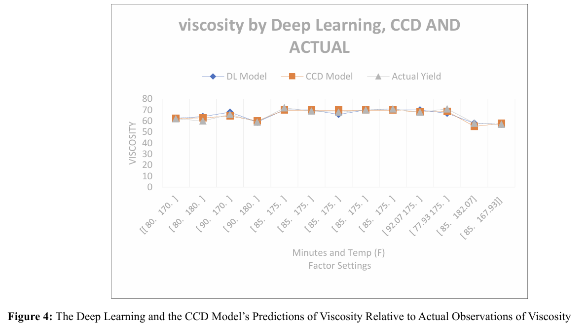
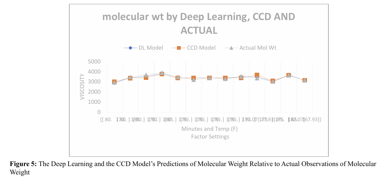
The effectiveness of the deep learning (DL) model building ap proach in comparison to the central composite design (CCD) based regression model can be evaluated in several ways. First ly, examining the model residuals in the last two columns of Table 2 reveals that each of the DL's residuals is smaller than the corresponding residual for the CCD model, even though we did not run the DL algorithm beyond a reasonable limit (epoch = 100000). This qualitative edge of DL over CCD is depicted graphically in Figure 3. Quantitatively, we observe that the root mean square error, which represents the standard deviation of the residuals, is 0.161209012 for DL, whereas it is 0.202432181 for the CCD model. We suggest that the DL model's apparent superior prediction performance is due to its ability to incorporate the response's true nonlinearities and higher order "terms" (which are attributable to the input factors, i.e., Time and Tem perature) more effectively. It is worth noting that the DL model's mean absolute error (MAE) is 0.119104923, indicating accept able predictive accuracy [11]. Furthermore, a chi-square test re vealed that the performance of CCD and DL were statistically indistinguishable for the present example. Figures 4 and 5 illus trate the predictions of process responses Viscosity and Molec ular Weight obtained by DL and CCD models, along with the actual experimental observations of those responses. The quality of these results is not substantially different from those observed for the response variable Yield.

Hyperparameter Tuning

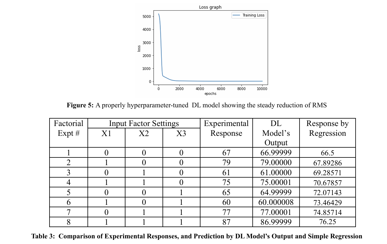
Perhaps the most taxing chore in building a reliable deep learn ing model from experimental data is tuning the hyperparameters of the model. Even when you feel that you have “cornered” the “optimal hyperparameters”, there will remain the challenge in achieving convergence without overtraining the model. One issue we repeatedly bumped into was setting the random seed, which determines the computational path taken by the heuristic global optimization. We conducted multiple trials with differ ent seeds and epochs to heuristically attain convergence while avoiding overtraining. No reliable guidelines are known to us as yet and the approach seems to rely greatly on hit and trial [5]. An example is given in Table 3 using data obtained from a 23 factorial experiment. Simple regression gave brutal predictions for it. The DL model was carefully developed by empirically optimizing the hyperparameters (see Figure 5). The gains of us ing deep learning to predict process outputs are quite prominent. Such results highlight the significance of careful and iterative tuning and optimization in the DL modeling approach.

Conclusions and Lessons Learned

This study offers valuable insights into the modeling of process es with input-output configurations. The following key lessons were learned:

• Modeling processes with input-output configurations has be come relatively straightforward with the availability of modern tools and devices such as deep learning. This study demonstrates how one can easily break into this highly rewarding world of ease and unexpected insights. Using a simple and compact code in Python (see the Appendix) incorporating some TensorFlow calls, we were able to optimize a real chemical engineering pro cess, surpassing the performance of reputed statistical experi mental designs.

• DL models can be built relatively easily using emergent com putational aids such as TensorFlow, Keras, Numpy, PyTorch, and others.

• Once built and tuned, DL models work very satisfactorily as substitutes for many relatively complex statistical techniques such as multiple regression and also reveal hidden nonlinearities.

• Gathering training data for ML/DL projects remains a daunt ing challenge. However, it is important to sample the application domain thoroughly, reaching into every corner of interest. This helps in probing areas and factor setting combinations where complex factor effect interactions may be concealed but active in the process. In many cases where nonlinearities are suspected to be present, conventional experimental schemes such as fraction al or even full factorial experimental designs may not be enough. This is a major limitation of even CCD and Box-Behnken statis tical experimental schemes. The authors recommend employing grid search in critical situations, even if conducting such experi ments could become expensive [3].

• Tuning the hyperparameters of the learning models built may present particular challenges. For instance, the model may give no indication that its performance is being grossly affected by the choice of the random seed set in the code. Such experiences are not uncommon, as learning models including DL have yet to become robust.

Summarily, we view that the proposed DL model provides a novel way to design statistically a process experiment of a man ufacturing system based on a benchmark problem obtained from a classical and significant author. On the other hand, the effectiveness of the DL measure is limited when the data is in accurate or hard to collect. The proposed method uses a novel concept which makes it unique and better than contemporary CCD methods. In order to further investigate the efficacy of the proposed model, some real-world case studies need to be carried out. Another direction of future research is to link the actual pro duction systems to further pinpoint the potential improvement opportunities. Finally, we submit that there is ample scope for expanding the literature regarding refinements of our articula tions and postulations and bringing analytical rigours. However, we have used the pragmatic research philosophy by integrating some ideas and innovations towards enriching the state-of-the art in Data Science discipline, which is facilitating more rapid ly to our broader field of knowledge in Industrial Engineering. Even then, in terms of towards the finality in refinement of the modelling and analysis, we make no claim but surely we enrich the profession.

References

1. Maran, J. P., Sivakumar, V., Thirugnanasambandham, K., & Sridhar, R. (2013). Artificial neural network and response surface methodology modeling in mass transfer parameters predictions during osmotic dehydration of Carica papaya L. Alexandria Engineering Journal, 52(3), 507-516.

2. IIT Kanpur (2023). Deep Learning Library

3. Montgomery, D. C. (2017). Design and analysis of experi ments. John wiley & sons.

4. Villarrubia, G., De Paz, J. F., Chamoso, P., & De la Prieta, F. (2018). Artificial neural networks used in optimization problems. Neurocomputing, 272, 10-16.

5. Pannakkong, W., Thiwa-Anont, K., Singthong, K., Part hanadee, P., & Buddhakulsomsiri, J. (2022). Hyperparam eter tuning of machine learning algorithms using response surface methodology: a case study of ANN, SVM, and DBN. Mathematical problems in engineering, 2022, 1-17.

6. Gupta, Sakshi (2022). AI vs. Machine Learning vs. Deep Learning: What’s the Difference?

7. Zhang, A., Lipton, Z. C., Li, M., & Smola, A. J. (2023). Dive into deep learning. Cambridge University Press.

8. Karazi, S. M., Issa, A., & Brabazon, D. (2009). Comparison of ANN and DoE for the prediction of laser-machined mi cro-channel dimensions. Optics and Lasers in Engineering, 47(9), 956-964.

9. Kafritsas, Nicolos (2023). Time-Series Forecasting: Deep Learning vs Statistics — Who Wins?

10. Snoek, J., Larochelle, H., & Adams, R. P. (2012). Practical bayesian optimization of machine learning algorithms. Ad vances in neural information processing systems, 25. 11. Mean Absolute Error ~ MAE [Machine Learning (ML)] (2023).

Appendix: A Prototype TensorFlow Code for Deep Learning

# -*- coding: utf-8 -*-
"""
Created on Wed Apr 12 21:52:30 2023
@author: lenovo
"""

import numpy as np
from tensorflow.keras.models import Sequential
from tensorflow.keras.layers import Dense
import tensorflow as tf

# Set up the input data
x = np.array([[0, 0, 0], [1, 0, 0], [0, 1, 0], [1, 1, 0], [0, 0, 1], [1, 0, 1], [0, 1, 1], [1, 1, 1]])
y = np.array([[67], [79], [61], [75], [65], [60],[77], [87]])

import random
tf.random.set_seed(987654)

#model defination
#Some hyperparameters we can tune to observe include

# 1. Changing the the number of input layer nodes and using non-linear activation function for the nodes. we can test from Relu to Tanh or sigmoid

model = Sequential()

model.add(Dense(10, input_dim=3, activation='relu'))

#model.add(Dense(20, input_dim=3, activation='tanh'))

model.add(Dense(24, activation='relu'))

#model.add(Dense(44, activation='tanh'))

model.add(Dense(1, activation='linear'))

# We can also change the learning rate to see what effects are revealed

model.compile(optimizer=tf.keras.optimizers.Adam(learning_rate=0.001), metrics=[tf.keras.metrics.RootMeanSquaredError()])

#model.compile(optimizer=tf.keras.optimizers.Adam(learning_rate=0.003), loss='mean_squared_error', metrics=[tf.keras.metrics.RootMeanSquaredError()])

model.summary()

# The number of epochs can also be changed

history= model.fit(x, y, batch_size=8, epochs=10000)

from matplotlib import pyplot as plt

plt.plot(history.history['loss'])

plt.title('Loss graph')

plt.xlabel('epochs')

plt.ylabel('loss')

plt.legend(['Training Loss'], loc=1)

loss= model.evaluate(x, y, verbose=0)

#print(f"Loss: {loss:.4f}")

print(loss)

# Predict on new data

new_data = np.array([[0, 0, 0], [1, 0, 0], [0, 1, 0], [1, 1, 0], [0, 0, 1], [1, 0, 1], [0, 1, 1], [1, 1, 1]])

predictions = model.predict(new_data)

print(predictions)

model.predict(x)

# Evaluate the model

loss, rmse = model.evaluate(x, y, verbose=0)

print(f"Loss: {loss:.4f}, Root_Mean_SQ_error: {rmse:.4f}")

# Predict on new data

new_data = np.array([[0, 0, 0], [1, 0, 0], [0, 1, 0], [1, 1, 0], [0, 0, 1], [1, 0, 1], [0, 1, 1], [1, 1, 1]])

predictions = model.predict(new_data)

print(predictions)